`<center>`07-给定区域WW3试验（2022寒假安排）`</center>`

文档托管

git托管：【https://github.com/Liu-Jincan/Data-Assimilation-for-Ocean-Current-Forecasts】
百度网盘托管：【】

—————————————CCMP

参考资料

官网：https://www.remss.com/measurements/ccmp/

2022-01-17 可以打开

CCMP Wind Vector Analysis Product

https://data.remss.com/ccmp/

2022-02-04 可以打开

来自于Wjc老师发的网站；

readme_ccmp.pdf 来自于 CCMP Wind Vector Analysis Product；

CCMP Wind Vector Analysis Product (2022-01-17)

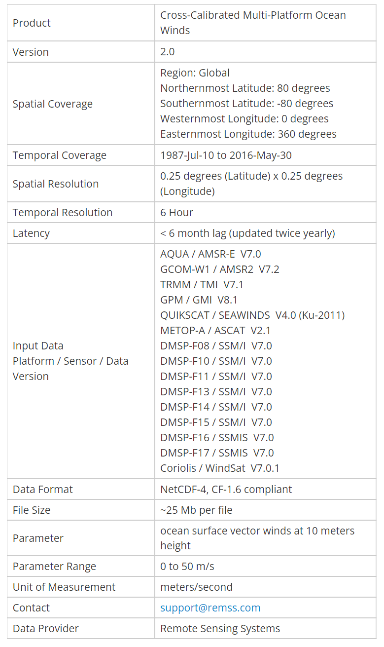
Version 2 CCMP Wind Product

The Cross-Calibrated Multi-Platform (CCMP) gridded surface vector winds are produced using satellite, moored buoy, and model wind data, and as such, are considered to be a Level-3 ocean vector wind analysis product. We have updated the CCMP product, using improved and additional input data.

This web site documents the new CCMP V2.0 data set now available from Remote Sensing Systems (RSS).

The V2 CCMP processing now combines Version-7 RSS radiometer wind speeds, QuikSCAT and ASCAT scatterometer wind vectors, moored buoy wind data, and ERA-Interim model wind fields using a Variational Analysis Method (VAM) to produce four maps daily of 0.25 degree gridded vector winds.

讲了此数据，用到了哪些数据，用什么方法。

The original CCMP product (V1.1) was originally produced by Bob Atlas and his team with funding from the NASA REASoN and MEaSUREs programs. The original MEaSUREs product is still available from the NASA Physical Oceanography DAAC (podaac.jpl.nasa.gov).

RSS has transitioned the CCMP processing code to run using our most up-to-date satellite data observations. All methodology remains the same as that used in the original CCMP product and most of the CCMP processing code is unchanged, with only minor alterations to compensate for the different operating systems and compilers.

transition 转换

compensate 补偿

Introduction

Gap-free ocean surface wind data of high quality and high temporal and spatial resolution are useful for a variety of purposes and are necessary for studying large scale air-sea interactions affecting the atmosphere and the ocean. Ocean vector winds are dynamic, continually evolving over short time scales. This characteristic makes the production of global, gridded, gap-free wind fields a challenge, especially at temporal scales of less than one day and spatial scales smaller than typical wind features.

Accurate research requires ocean vector wind data for a long enough time period to resolve wind-induced patterns such as the El Niño-Southern Oscillation (ENSO) and the Madden-Julian Oscillation (MJO). Remote Sensing Systems has invested many years of research into validating and cross-calibrating passive and active microwave wind retrievals from satellites.

介绍了数据应该需要反应相关现象；

passive 被动的

retrieval 挽回

The Variational Analysis Method (VAM) of data assimilation was utilized by Atlas et al. [1996, 2011] to find the most dynamically suitable way to combine satellite observations and in situ wind measurements into gap-free wind fields. The VAM generates a gridded surface wind analysis which minimizes an objective function measuring the misfit of the analysis to the background, the data and certain a priori constraints.

介绍VAM方法及其作用；

The CCMP wind analyses are at temporal and spatial resolutions suitable for scientific study. The CCMP Version 2.0 (V2) data product described here is a continuation of the highly-used original CCMP product (V1.1 available from NASA JPL PO.DAAC) and builds on the decades of careful VAM development. Two peer-reviewed publications (Atlas et al. 1996, Atlas et al., 2011) describe the original CCMP product and (Hoffman et al, 2003) describes the VAM. This documentation describes the new CCMP V2.0 product available from Remote Sensing Systems.

The original V1.1 CCMP product was processed incrementally, over a number of years, in small batches using the satellite data available at the time of processing, and therefore, <font color='red'>assimilated inconsistently processed satellite winds</font>. That is, earlier V4 through V6 RSS winds were used for early production years with V7 winds for the later few years of production. Funding for the original CCMP (V1.1) ended in 2012 with no CCMP winds produced since December 2011. There has been considerable demand for the continuation of the CCMP product, so we have transitioned the code to RSS with the purpose of meeting several distinct goals:

Extend the product to the present time and continue processing into the future.
Reprocess using a consistent version of satellite data.
Add newly available sensors.
Utilize a higher resolution and consistently produced background model wind field throughout the analysis product.

incrementally 递增的

We provide the Level-3.0 (L3.0) and Level-3.5 (L3.5) CCMP V2.0 products in netCDF4 format.

The L3.0 CCMP V2.0 product contains four daily maps (00, 06, 12, and 18Z) of U and V vector wind components on a 0.25 degree global grid. The U and V components are relative to true north. The L3.0 data also includes maps of the number of observations (both satellite and in situ) that were analyzed at each location.
The L3.5 CCMP V2.0 contains monthly winds averaged over the calendar month. Vector averages are computed for U and V. The average wind W is computed using a scalar average.
Updates to the CCMP V2.0 product will be made roughly twice a year, to complete processing through December and June.
The most recent update occurred in March 2018, and CCMP is now updated through December 30, 2017.

Product Development

The CCMP data set combines cross-calibrated satellite microwave winds and instrument observations using a Variational Analysis Method (VAM) to produce high-resolution (0.25 degree) gridded analyses.

Satellite wind retrievals derived by Remote Sensing Systems from a number of satellite-borne passive and active microwave instruments are used. RSS intercalibrates radiometers at the brightness temperature level to within 0.2 degree Celsius, applying a refined sea-surface emissivity model and radiative transfer function to derive surface winds. The resulting wind retrievals are highly consistent between microwave radiometer instrument platforms, including SSM/I, SSMIS, AMSR, TMI, WindSat, and GMI. RSS has also developed a geophysical model function for deriving wind speeds and directions from microwave scatterometers, including QuikSCAT and ASCAT.

Both radiometer and scatterometer data are validated against ocean moored buoys, which confirm the measurements are in agreement (to within 0.8 m/s) despite the difference in wind measurement and retrieval methodologies.

The VAM combines RSS instrument data with moored buoy measurements and a starting estimate (first-guess) of the wind field.

The European Center for Medium-Range Weather Forecasts (ECMWF) ERA-Interim Reanalysis winds are used in the CCMP V2.0 processing as the first-guess wind field. This 0.25 deg model wind field is consistently processed, as opposed to that of the ECMWF operational model for which the model changes over time.

All wind observations (satellite and buoy) and model analysis fields are referenced to a height of 10 meters.

CCMP VERSION-2 UPDATES

RSS cooperated with Dr. Ross Hoffman and Mark Leidner to transition the maintenance, update, and continued processing of CCMP. Once the transition was confirmed to be accurately functioning, RSS conducted a full reprocessing of the CCMP data set bringing it out of first-look status and delivering a consistently-reprocessed V2.0 data product for public use in scientific research. The version changes associated with the RSS V2.0 CCMP release include:

Use of uniform inputs and satellite retrievals, with all satellite winds produced using RSS Version-7 (or higher) Ocean Radiative Transfer Model (ORTM) and a consistent processing methodology.
Extension of the CCMP data set to July 2015 with plans to provide bi-annual extensions and updates to the dataset.
Addition of winds from new instruments: ASCAT Metop-A, AMSR2, and GMI.
Upgrade of the first-guess background wind field. Now using the 0.25-deg, 6-hourly ERA-Interim Reanalysis winds.
Use of improved moored buoy data with better quality control, including winds from NDBC, TAO, TRITON, RAMA, PIRATA, and Canadian buoys.
Upgrade of the data file format to netCDF4 with CF-1.6 metadata. Each daily file contains four 6-hourly wind analyses and self-describing metadata.

A time series of all input data used in the VAM is shown below. Passive radiometers are plotted in red and active scatterometers are plotted in green. The version of data used for each instrument is provided. The moored buoy winds and ERA-Interim Reanalysis winds are available for the entire data range. Quality controlled buoy data have been obtained from the Pacific Marine Environmental Lab (PMEL), from the National Data Buoy Center (NDBC), and from the Fisheries and Ocean Canada Oceanography and Scientific Data branch (OSD).

Full reprocessing of the entire data set takes approximately 1-2 months. Twice per year, in January and July, we will update the data product to include the past 6 months. For example, in January 2017, we will release June 2016 to December 2016. In transitioning the code to run at RSS, special care was taken to make no changes to the overall approach or the methodology of the original CCMP product. The code was changed, only where necessary, to account for changes in system architecture and compilers. Source code that was needed for the addition of new satellite winds (AMSR2 or GMI) was adapted from already existing code. This type of careful transition ensures that the same high-quality CCMP product is still produced, but with updated satellite, buoy and model wind data as input.

Data Product Format

The CCMP V2.0 Level-3.0 (L3.0) winds are available as netCDF-4 data files. Each L3.0 daily data file contains 3 arrays of size 1440 (longitude) by 628 (latitude for range -78.375 to 78.375) by 4 (time of 0Z, 06Z, 12Z, 18Z). Two of the arrays are the U and V wind components in meters/second (m/s). Standard U and V coordinates apply, meaning the positive U is to the right and positive V is above the axis. U and V are relative to true north. CCMP winds are expressed using the oceanographic convention, meaning a wind blowing toward the Northeast has a positive U component and a positive V component. The third array in the file is the number of observations (nobs) used to derive the wind components. A nobs value of 0.0 means that the wind vector for that grid cell is very close to the wind vector from the background field because no satellite or moored buoy wind data were available to directly influence the analyzed vector wind.

The CCMP V2.0 Level-3.5 (L3.5) winds are available as netCDF-4 data files. Each L3.5 monthly data file contains 3 arrays of size 1440 (longitude) by 628 (latitude for range -78.375 to 78.375) by 1 (time centered on the middle of the calendar month). The first two arrays are the vector-averaged U and V wind components in meters/second (m/s). The third array contains the scalar-averaged wind speed W for each location. Note that in regions with wind directions that vary substantially over time, W can be much higher than the magnitude of the vector-average components U and V.

A fill value of -9999.0 is used for any grid cell without any data. This should rarely happen. Longitude is given in degrees East from 0.125 to 359.875 and latitude is given in degrees North with negative values representing southern locations. While this is referred to as a global wind product, the extent of the data is -79 degrees to 79 degrees latitude. The time in the file is given as hours since midnight on Jan 1, 1987.

The netCDF file contains CF 1.6-compliant self-describing metadata. The JPL metadata compliance checker was used to assess compliance. The RSS CCMP V2.0 data set is distributed as L3.0 daily and L3.5 monthly files. The V1.1 CCMP data set available from PO.DAAC also contained L2.5 (vectors on satellite data) and L3.5 pentad data products. However, RSS has chosen to not distribute the L2.5 or L3.5 pentad data products at this time.

MISSING DATA

There are gaps within these data. There are 11 days scattered between May and December of 1988 and 14 days in January through July 1989 that do not appear on our FTP server

During this time period, F08 is the only operational satellite input into the dataset. Days that are missing are because there was either very little or no data collected by the satellite on that day.

In future reprocessing, we may include these files for completeness, but the CCMP wind field would essentially be just the ERA-Int background except for minor differences near buoys.

Read Routines / Data Access

The CCMP netCDF4 files can be explored using tools such as Panoply or ncBrowse. Matlab, IDL, and Python have built-in routines for reading netCDF files. We have provided a sample read routine in Python. The routine will plot and display the data for an example file. CCMP data files can be obtained from RSS by ftp and http.

remss：remote sensing system

File names have the structure CCMP_Wind_Analysis_YYYYMMDD_V02.0_L3.0_RSS.nc where YYYY is the 4-digit year, MM the month and DD the day-of-month. The files are stored in v02.0/Yyyyy/Mmm/ directory structure.

Browse Images / Graphic Maps

The following movies loop through the full 28 years of data.

CCMP Wind Speed Animation

已上传至个人B站：

CCMP Wind Speed Anomaly Animation

已上传至个人B站：

Product Details

Known Issues / Data Caveats

The following information should be taken into consideration when using this data product:

Users should not consider these winds suitable for studying global trends. While the winds are derived from consistently processed satellite data suitable for climate study, the act of assimilating the model data into an analysis product potentially introduces spurious trends that may exist in the background wind field. These CCMP V2.0 winds may, however, be suitable for studying regional trends and patterns.
Caution should be used when studying high wind regions. We have noted differences between satellite data and the CCMP winds at high wind speeds (>25 m/s), where the background model wind is known to underestimate wind events. Since the VAM method attempts to find a consistent wind field solution somewhere between the satellite-observed high wind events and the lower model winds for those same events, CCMP, as a wind analysis product, will inevitably be lower than the satellite data indicates. Note, wind events of this magnitude tend to be infrequent and geographically limited.
The V2.0 winds are different from the V1.1 winds. Users should not compare or mix the two products. Differences between the versions do exist and are related to the changes in the satellite data and background wind field. For example, the new Ku-2011 GMF QuikSCAT winds are much improved at high wind speeds resulting in lower CCMP V2.0 winds at speeds greater than 25 m/s when compared to the CCMP V1.1 winds.

The original CCMP V1.1 FLK data are available at the NASA Physical Oceanography DAAC (podaac.jpl.nasa.gov)

References

Atlas, R., R. N. Hoffman, J. Ardizzone, S. M. Leidner, J. C. Jusem, D. K. Smith, D. Gombos, 2011: A cross-calibrated, multiplatform ocean surface wind velocity product for meteorological and oceanographic applications. Bull. Amer. Meteor. Soc., 92, 157-174. doi: 10.1175/2010BAMS2946.1

Atlas, R., R.N. Hoffman, S.C. Bloom, J.C. Jusem, and J. Ardizzone, 1996: A multiyear global surface wind velocity dataset using SSM/I wind observations. Bull. Amer. Meteor. Soc., 77, 5, 869-882.

Hoffman, R. N., M. Leidner, J. M. Henderson, R. Atlas, J. V. Ardizzone, and S. C. Bloom, 2003: A two-dimensional variational analysis method for NSCAT ambiguity removal: methodology, sensitivity, and tuning. Journal of Atmospheric & Oceanic Technology, 20, 585-605.

The original V1.1 Cross-Calibrated Multi-Platform Ocean Surface Wind Vector Analyses User Guide (.pdf) available from JPL PO.DAAC.

How to Cite These Data

Continued production of this data set requires support from NASA. We need you to be sure to cite these data when used in your publications so that we can demonstrate the value of this data set to the scientific community. Please include the following statement in the acknowledgement section of your paper:

“CCMP Version-2.0 vector wind analyses are produced by Remote Sensing Systems. Data are available at www.remss.com.”

DATA SET CITATION

Wentz, F.J., J. Scott, R. Hoffman, M. Leidner, R. Atlas, J. Ardizzone, 2015: Remote Sensing Systems Cross-Calibrated Multi-Platform (CCMP) 6-hourly ocean vector wind analysis product on 0.25 deg grid, Version 2.0, [indicate date subset, if used]. Remote Sensing Systems, Santa Rosa, CA. Available online at www.remss.com/measurements/ccmp. [Accessed dd mmm yyyy]. *Insert the appropriate information in the brackets.

JOURNAL REFERENCE

Mears, C. A., Scott, J., Wentz, F. J., Ricciardulli, L., Leidner, S. M., Hoffman, R., & Atlas, R. ( 2019). A Near Real Time Version of the Cross Calibrated Multiplatform (CCMP) Ocean Surface Wind Velocity Data Set. Journal of Geophysical Research: Oceans, 124, 6997– 7010. https://doi.org/10.1029/2019JC015367

参考资料

https://blog.csdn.net/qq_38882446/article/details/111371015

matlab, web 函数

http://blog.sina.com.cn/s/blog_aed5bd1d0102wusz.html

matlab, urlwrite 函数

https://www.ilovematlab.cn/thread-253224-1-1.html?s_tid=RelatedContent

matlab，判断选择的日期不存在

下载CCMP数据（matlab, urlwrite 函数）

下载所需程序 download_ccmp.m：

%% 说明
% ccmp v02.0 数据下载网址：https://data.remss.com/ccmp/v02.0/


%% L3.0数据下载
filepath='D:\ccmp\data_L3\'; mkdir(filepath); %创建相应文件夹，下载的数据保存到此文件夹；(注意，路径的最后面必须为 \ )；

% url特点：需要3个通配符
% https://data.remss.com/ccmp/v02.0/Y1990/M02/CCMP_Wind_Analysis_19900201_V02.0_L3.0_RSS.nc
%                                    1987:1:2019
%                                          01:1:12
%                                                                          01:1:31

% 最全的通配符
% year = num2str([1987:1:2019]');  year(2,:); size(year);%通配符 year；
% month = num2str([1:1:12]','%02d'); month(2,:); %通配符 month；
% day = num2str([1:1:31]','%02d'); day(2,:); %通配符 day；

% 应用中的通配符
year = num2str([2011]'); %通配符 year；
month = num2str([9]','%02d'); %通配符 month；
day = num2str([1:10]','%02d'); %通配符 day；

for i=1:1:size(year,1)
    for j=1:1:size(month,1)
        for k=1:1:size(day,1)
            % 判断日期存不存在
            ts = [year(i,:),'-',month(j,:),'-',day(k,:)];
            try
                tf = isdatetime(datetime(ts)); %不用try，这一行会报错。
            catch
                tf = 0;
            end
          
            if(tf==1) %日期存在
                %https://data.remss.com/ccmp/v02.0/Y1990/M02/CCMP_Wind_Analysis_19900201_V02.0_L3.0_RSS.nc
                fullURL=['https://data.remss.com/ccmp/v02.0/Y',year(i,:), ...
                    '/M',month(j,:), ...
                    '/CCMP_Wind_Analysis_',year(i,:),month(j,:),day(k,:),'_V02.0_L3.0_RSS.nc']; %下载所需要的url
                filename=[filepath,'CCMP_Wind_Analysis_',year(i,:),month(j,:),day(k,:),'_V02.0_L3.0_RSS.nc']; %保存的文件名
              
                tic % 记录下载的时间
                [f,status]=urlwrite(fullURL,filename);%下载命令
                if status==1 %下载成功
                    t=toc;
                    lst=dir(filename); %了解文件的大小
                    xi=lst.bytes;
                    disp(['CCMP_Wind_Analysis_',year(i,:),month(j,:),day(k,:),'_V02.0_L3.0_RSS.nc',...
                        '下载成功，','文件大小为',num2str(xi/1024/1024),'M，',' 花费',num2str(t/60),'分钟。']);
                else
                    disp(['CCMP_Wind_Analysis_',year(i,:),month(j,:),day(k,:),'_V02.0_L3.0_RSS.nc','下载失败。']);
                end
            else
                disp([ts,'日期不存在。']);
            end
          
        end
    end
end

%% L3.5数据下载
% ...

运行程序后，会下载20110901-20110910的数据，可以根据自己需求改变时间段。

参考资料

https://blog.csdn.net/schumacher2016/article/details/82852700

多个netcdf文件的合并（matlab）

https://blog.csdn.net/muse_squirrel/article/details/76014446

Matlab 查阅、读取nc数据

https://ww2.mathworks.cn/help/matlab/ref/netcdf.redef.html

netcdf.reDef

合并CCMP的nc数据（matlab）

查阅某一个CCMP的nc文件，matlab输出如下：

>> ncdisp(strcat(datadir,filelist(i).name),'/','full')
Source:
           D:\ccmp\data_L3\CCMP_Wind_Analysis_20110902_V02.0_L3.0_RSS.nc
Format:
           netcdf4_classic
Global Attributes:
           contact                   = 'Remote Sensing Systems, support@remss.com'
           Conventions               = 'CF-1.6'
           data_structure            = 'grid'
           title                     = 'RSS CCMP V2.0 derived surface winds (Level 3.0)'
           history                   = '20160212T164116ZZ - netCDF generated from original data using MATLAB 8.5.0 by RSS vam_v2.0.analysis.t20110902.z00.dat; vam_v2.0.analysis.t20110902.z06.dat; vam_v2.0.analysis.t20110902.z12.dat; vam_v2.0.analysis.t20110902.z18.dat'
           description               = 'RSS VAM 6-hour analyses starting from the ERA-Interim wind analyses'
           summary                   = 'CCMP V2.0 has been created using the same VAM as CCMP V1.1 only it is now running at Remote Sensing Systems. Input data have changed and now include all V7 radiometer data from RSS, V8.1 GMI data from RSS, scatterometer data from RSS (V4 QuikSCAT and V1.2 ASCAT), quality checked moored buoy data from NDBC, PMEL, and ISDM, and ERA-Interim data from ECMWF.'
           institute_id              = 'RSS'
           institution               = 'Remote Sensing Systems (RSS)'
           base_date                 = 'Y2011 M09 D02'
           comment                   = 'none'
           license                   = 'available for public use with proper citation'
           product_version           = 'v2.0'
           netcdf_version_id         = '4.2'
           date_created              = '20160212T164116Z'
           geospatial_lat_units      = 'degrees_north'
           geospatial_lat_resolution = '0.25 degrees'
           geospatial_lat_min        = '-78.375 degrees'
           geospatial_lat_max        = '78.375 degrees'
           geospatial_lon_units      = 'degrees_east'
           geospatial_lon_resolution = '0.25 degrees'
           geospatial_lon_min        = '0.125 degrees'
           geospatial_lon_max        = '359.875 degrees'
           creator_name              = 'Remote Sensing Systems'
           creator_email             = 'support@remss.com'
           creator_url               = 'http://www.remss.com/'
           project                   = 'RSS Cross-Calibrated Multi-Platform Ocean Surface Wind Project'
           publisher_name            = 'Remote Sensing Systems'
           publisher_email           = 'support@remss.com'
           publisher_url             = 'http://www.remss.com/'
           contributor_name          = 'Joel Scott, Frank Wentz, Ross Hoffman, Mark Leidner, Robert Atlas, Joe Ardizzone'
           contributor_role          = 'Software Engineer, Project Lead, Co-Investigator, Software Engineer, Principal Investigator, Software Engineer'
           processing_level          = 'L3.0'
           keywords                  = 'surface winds, ocean winds, wind speed/wind direction, MEaSUREs, 10km - < 50km or approximately 0.09 degree - < 0.5 degree'
           keywords_vocabulary       = 'GCMD Science Keywords'
           references                = 'Hoffman et al., Journal of Atmospheric and Oceanic Technology, 2013; Atlas et al., BAMS, 2011; Atlas et al., BAMS, 1996'
Dimensions:
           longitude = 1440
           latitude  = 628
           time      = 4
Variables:
    longitude
           Size:       1440x1
           Dimensions: longitude
           Datatype:   single
           Attributes:
                       standard_name       = 'longitude'
                       long_name           = 'Longitude in degrees east'
                       units               = 'degrees_east'
                       _Fillvalue          = -9999
                       axis                = 'X'
                       valid_min           = 0.125
                       valid_max           = 359.875
                       _CoordinateAxisType = 'Lon'
                       coordinate_defines  = 'center'
    latitude 
           Size:       628x1
           Dimensions: latitude
           Datatype:   single
           Attributes:
                       standard_name       = 'latitude'
                       long_name           = 'Latitude in degrees north'
                       units               = 'degrees_north'
                       _Fillvalue          = -9999
                       axis                = 'Y'
                       valid_min           = -78.375
                       valid_max           = 78.375
                       _CoordinateAxisType = 'Lat'
                       coordinate_defines  = 'center'
    time   
           Size:       4x1
           Dimensions: time
           Datatype:   double
           Attributes:
                       standard_name       = 'time'
                       long_name           = 'Time of analysis'
                       units               = 'hours since 1987-01-01 00:00:00'
                       delta_t             = '0000-00-00 06:00:00'
                       avg_period          = ''
                       _Fillvalue          = -9999
                       calendar            = 'standard'
                       axis                = 'T'
                       valid_min           = 216240
                       valid_max           = 216258
                       _CoordinateAxisType = 'Time'
    uwnd   
           Size:       1440x628x4
           Dimensions: longitude,latitude,time
           Datatype:   single
           Attributes:
                       standard_name = 'eastward_wind'
                       long_name     = 'u-wind vector component at 10 meters'
                       units         = 'm s-1'
                       height        = '10 meters above sea-level'
                       _Fillvalue    = -9999
                       valid_min     = -29.0874
                       valid_max     = 28.8251
                       coordinates   = 'time latitude longitude'
    vwnd   
           Size:       1440x628x4
           Dimensions: longitude,latitude,time
           Datatype:   single
           Attributes:
                       standard_name = 'northward_wind'
                       long_name     = 'v-wind vector component at 10 meters'
                       units         = 'm s-1'
                       height        = '10 meters above sea-level'
                       _Fillvalue    = -9999
                       valid_min     = -23.203
                       valid_max     = 32.6429
                       coordinates   = 'time latitude longitude'
    nobs   
           Size:       1440x628x4
           Dimensions: longitude,latitude,time
           Datatype:   single
           Attributes:
                       standard_name       = 'number_of_observations'
                       long_name           = 'number of observations used to derive wind vector components'
                       units               = 'count'
                       _Fillvalue          = -9999
                       ancillary_variables = 'uwnd vwnd'
                       valid_min           = 0
                       valid_max           = 10
                       coordinates         = 'time latitude longitude'

这里给出将20110901-20110910的nc文件合并的程序 merge_ccmp.m，可以根据自己需求改变相关参数：

%%
% desciption: merge multiple netcdf files for sepcific domain

% usage:
%    1. filenumber is up to the number of your netcdf file to be processed.
%    2. for different domain you want to process, you can change the number
% in the latitude0, longitude0, uwind0, vwind0.

% author:
%    huang xue zhi, dalian university of technology

% revison history
%    2018-09-25 first verison.

%%
clear;clc;

% begin to merge multiple netcdf files,for example,ccmp wind field reanalysis.



% define the data path and filelist
datadir='D:\ccmp\data_L3\';
filelist=dir([datadir,'*.nc']); 
% define the total numbers of netcdf files to be processed.
filenumber=size(filelist,1); %全部nc文件的数量

%% batch reading from the netcdf file
for i=1:filenumber
    % 查阅nc相关信息
    %ncdisp(strcat(datadir,filelist(i).name),'/','min')
    %ncdisp(strcat(datadir,filelist(i).name),'/','full')
  
    % batch reading the variable to another arrays.
    ncid=[datadir,filelist(i).name];
  
    latitude0=ncread(ncid,'latitude'); %0.25间隔
    longitude0=ncread(ncid,'longitude'); %0.25间隔
    time(:,i)=ncread(ncid,'time');       % 增加了数组维数，保留信息。
    uwind0(:,:,:,i)=ncread(ncid,'uwnd'); % 增加了数组维数，保留信息。
    vwind0(:,:,:,i)=ncread(ncid,'vwnd'); % 增加了数组维数，保留信息。
  
    %区域纬度的选择
    %latitude=latitude0(74:435);
    %longitude=longitude0(80:481);
    %uwind(:,:,:,i)=uwind0(80:481,74:435,:,i);
    %vwind(:,:,:,i)=vwind0(80:481,74:435,:,i);
    latitude=latitude0;
    longitude=longitude0;
    uwind=uwind0;
    vwind=vwind0;
end

%% create the merged netcdf file to store the result.
filename = 'ccmp20110901to10.nc'; %合成的nc文件名称
cid=netcdf.create(filename,'clobber'); % help netcdf.create


%define global attributes
netcdf.putAtt(cid,netcdf.getConstant('NC_GLOBAL'),'Conventions','CF-1.6'); % help netcdf.putAtt
netcdf.putAtt(cid,netcdf.getConstant('NC_GLOBAL'),'geospatial_lat_min','-78.375 degrees');
netcdf.putAtt(cid,netcdf.getConstant('NC_GLOBAL'),'geospatial_lat_max','78.375 degrees');
netcdf.putAtt(cid,netcdf.getConstant('NC_GLOBAL'),'geospatial_lon_min','0.125 degrees');
netcdf.putAtt(cid,netcdf.getConstant('NC_GLOBAL'),'geospatial_lon_max','359.875 degrees');
netcdf.putAtt(cid,netcdf.getConstant('NC_GLOBAL'),'institution','RSS');

% define the variable dimension
dimlon=netcdf.defDim(cid,'longitude',size(longitude,1));
dimlat=netcdf.defDim(cid,'latitude',size(latitude,1));
dimtime=netcdf.defDim(cid,'time',filenumber*4); %每天有4个时间结点


% define the variable and their attributes
varid1=netcdf.defVar(cid,'time','NC_DOUBLE',dimtime);
netcdf.putAtt(cid,varid1,'standard_name','time');
netcdf.putAtt(cid,varid1,'long_name','Time of analysis');
netcdf.putAtt(cid,varid1,'units','hours since 1987-01-01 00:00:00');
netcdf.putAtt(cid,varid1,'delta_t','0000-00-00 06:00:00');

varid2=netcdf.defVar(cid,'latitude','NC_FLOAT',dimlat);
netcdf.putAtt(cid,varid2,'standard_name','time');
netcdf.putAtt(cid,varid2,'units','degrees_north');
netcdf.putAtt(cid,varid2,'long_name','Latitude in degrees north');
netcdf.putAtt(cid,varid2,'_Fillvalue','-9999.0');
netcdf.putAtt(cid,varid2,'axis','Y');


varid3=netcdf.defVar(cid,'longitude','NC_FLOAT',dimlon);
netcdf.putAtt(cid,varid3,'standard_name','longitude');
netcdf.putAtt(cid,varid3,'units','degrees_east');
netcdf.putAtt(cid,varid3,'long_name','Longitude in degrees east');
netcdf.putAtt(cid,varid3,'_Fillvalue','-9999.0');
netcdf.putAtt(cid,varid3,'axis','X');


varid4=netcdf.defVar(cid,'u10','NC_FLOAT',[dimlon dimlat dimtime]);
netcdf.putAtt(cid,varid4,'standard_name','eastward_wind');
netcdf.putAtt(cid,varid4,'long_name','u-wind vector component at 10 meters');
netcdf.putAtt(cid,varid4,'units','m s-1');
netcdf.putAtt(cid,varid4,'_Fillvalue','-9999.0');
netcdf.putAtt(cid,varid4,'coordinates','time latitude longitude')


varid5=netcdf.defVar(cid,'v10','NC_FLOAT',[dimlon dimlat dimtime]);
netcdf.putAtt(cid,varid5,'standard_name','northward_wind');
netcdf.putAtt(cid,varid5,'long_name','v-wind vector component at 10 meters');
netcdf.putAtt(cid,varid5,'units','m s-1');
netcdf.putAtt(cid,varid5,'_Fillvalue','-9999.0');
netcdf.putAtt(cid,varid5,'coordinates','time latitude longitude')

netcdf.endDef(cid);
% end define the varible and attributes


%% write variables value to merged netcdf file
netcdf.putVar(cid,varid1,time);
netcdf.putVar(cid,varid2,latitude);
netcdf.putVar(cid,varid3,longitude);
netcdf.putVar(cid,varid4,uwind);
netcdf.putVar(cid,varid5,vwind);

% 添加存储空间属性
netcdf.reDef(cid); %data mode 不能进行使用 putAtt，故进入 def mode；
lst=dir(filename); xi=lst.bytes;
netcdf.putAtt(cid,netcdf.getConstant('NC_GLOBAL'),'space size',strcat(num2str(xi/1024/1024),'Mb'));
%ncdisp(filename,'/','full');

netcdf.close(cid);

运行后，将生成合并的nc文件 ccmp20110901to10.nc，查阅：

>> ncdisp(filename,'/','full')
Source:
           D:\ccmp\ccmp20110901to10.nc
Format:
           classic
Global Attributes:
           Conventions        = 'CF-1.6'
           geospatial_lat_min = '-78.375 degrees'
           geospatial_lat_max = '78.375 degrees'
           geospatial_lon_min = '0.125 degrees'
           geospatial_lon_max = '359.875 degrees'
           institution        = 'RSS'
           space size         = '275.9862Mb'
Dimensions:
           longitude = 1440
           latitude  = 628
           time      = 40
Variables:
    time   
           Size:       40x1
           Dimensions: time
           Datatype:   double
           Attributes:
                       standard_name = 'time'
                       long_name     = 'Time of analysis'
                       units         = 'hours since 1987-01-01 00:00:00'
                       delta_t       = '0000-00-00 06:00:00'
    latitude 
           Size:       628x1
           Dimensions: latitude
           Datatype:   single
           Attributes:
                       standard_name = 'time'
                       units         = 'degrees_north'
                       long_name     = 'Latitude in degrees north'
                       _Fillvalue    = '-9999.0'
                       axis          = 'Y'
    longitude
           Size:       1440x1
           Dimensions: longitude
           Datatype:   single
           Attributes:
                       standard_name = 'longitude'
                       units         = 'degrees_east'
                       long_name     = 'Longitude in degrees east'
                       _Fillvalue    = '-9999.0'
                       axis          = 'X'
    u10    
           Size:       1440x628x40
           Dimensions: longitude,latitude,time
           Datatype:   single
           Attributes:
                       standard_name = 'eastward_wind'
                       long_name     = 'u-wind vector component at 10 meters'
                       units         = 'm s-1'
                       _Fillvalue    = '-9999.0'
                       coordinates   = 'time latitude longitude'
    v10    
           Size:       1440x628x40
           Dimensions: longitude,latitude,time
           Datatype:   single
           Attributes:
                       standard_name = 'northward_wind'
                       long_name     = 'v-wind vector component at 10 meters'
                       units         = 'm s-1'
                       _Fillvalue    = '-9999.0'
                       coordinates   = 'time latitude longitude'

合并CCMP的nc数据（matlab，专门用于ww3_prnc）

用上面的代码，实现的合并的nc文件，在执行ww3_prnc时，会出现 Segmentation fault - invalid memory reference错误信息，与内存相关，原因是ww3_prnc中 _Fillvalue这一项应该是 _FillValue，且数值应该是 -9999，而不需要加上 ''。

直接使用ccmp的nc文件也会出现上述错误信息。

这里给出将20110901-20110910的nc文件，用于ww3_prnc，合并的程序 merge_ccmp_ww3.m：

%%
% desciption: merge multiple netcdf files for sepcific domain

% usage:
%    1. filenumber is up to the number of your netcdf file to be processed.
%    2. for different domain you want to process, you can change the number
% in the latitude0, longitude0, uwind0, vwind0.

% author:
%    huang xue zhi, dalian university of technology
%    liu jin can, UPC

% revison history
%    2018-09-25 first verison.
%    2022-02-10 ww3.

%%
clear;clc;

% begin to merge multiple netcdf files,for example,ccmp wind field reanalysis.



% define the data path and filelist
datadir='D:\ccmp\data_L3\';
filelist=dir([datadir,'*.nc']); 
% define the total numbers of netcdf files to be processed.
filenumber=size(filelist,1); %全部nc文件的数量

%% batch reading from the netcdf file
for i=1:filenumber
    % 查阅nc相关信息
    %ncdisp(strcat(datadir,filelist(i).name),'/','min')
    %ncdisp(strcat(datadir,filelist(i).name),'/','full')
  
    % batch reading the variable to another arrays.
    ncid=[datadir,filelist(i).name];
  
    latitude0=ncread(ncid,'latitude'); %0.25间隔
    longitude0=ncread(ncid,'longitude'); %0.25间隔
    time(:,i)=ncread(ncid,'time');       % 增加了数组维数，保留信息。
    uwind0(:,:,:,i)=ncread(ncid,'uwnd'); % 增加了数组维数，保留信息。
    vwind0(:,:,:,i)=ncread(ncid,'vwnd'); % 增加了数组维数，保留信息。
  
    %区域纬度的选择
    %latitude=latitude0(74:435);
    %longitude=longitude0(80:481);
    %uwind(:,:,:,i)=uwind0(80:481,74:435,:,i);
    %vwind(:,:,:,i)=vwind0(80:481,74:435,:,i);
    latitude=latitude0;
    longitude=longitude0;
    uwind=uwind0;
    vwind=vwind0;
end

%% create the merged netcdf file to store the result.
filename = 'wind10.nc'; %合成的nc文件名称

% cmode 选择，help netcdf.create
%cid=netcdf.create(filename,'clobber'); 
cid=netcdf.create(filename,'64BIT_OFFSET'); % 64BIT_OFFSET


%define global attributes
netcdf.putAtt(cid,netcdf.getConstant('NC_GLOBAL'),'Conventions','CF-1.6'); % help netcdf.putAtt
netcdf.putAtt(cid,netcdf.getConstant('NC_GLOBAL'),'data_structure','grid');
netcdf.putAtt(cid,netcdf.getConstant('NC_GLOBAL'),'geospatial_lat_min','-78.375 degrees');
netcdf.putAtt(cid,netcdf.getConstant('NC_GLOBAL'),'geospatial_lat_max','78.375 degrees');
netcdf.putAtt(cid,netcdf.getConstant('NC_GLOBAL'),'geospatial_lon_min','0.125 degrees');
netcdf.putAtt(cid,netcdf.getConstant('NC_GLOBAL'),'geospatial_lon_max','359.875 degrees');
netcdf.putAtt(cid,netcdf.getConstant('NC_GLOBAL'),'institution','Remote Sensing Systems (RSS)');

% define the variable dimension
dimlon=netcdf.defDim(cid,'longitude',size(longitude,1));
dimlat=netcdf.defDim(cid,'latitude',size(latitude,1));
dimtime=netcdf.defDim(cid,'time',filenumber*4); %每天有4个时间结点


% define the variable and their attributes
varid1=netcdf.defVar(cid,'time','NC_DOUBLE',dimtime); % help netcdf.defVar
netcdf.putAtt(cid,varid1,'standard_name','time');
netcdf.putAtt(cid,varid1,'long_name','Time of analysis');
netcdf.putAtt(cid,varid1,'units','hours since 1987-01-01 00:00:00');
netcdf.putAtt(cid,varid1,'delta_t','0000-00-00 06:00:00');
netcdf.putAtt(cid,varid1,'calendar','standard');
netcdf.putAtt(cid,varid1,'valid_min',min(time));
netcdf.putAtt(cid,varid1,'valid_max',max(time));
netcdf.putAtt(cid,varid1,'axis','T');

%varid2=netcdf.defVar(cid,'latitude','NC_FLOAT',dimlat);
varid2=netcdf.defVar(cid,'latitude','NC_DOUBLE',dimlat); % NC_DOUBLE 要求的内存，基本是 NC_FLOAT 的2倍
netcdf.putAtt(cid,varid2,'standard_name','latitude');
netcdf.putAtt(cid,varid2,'units','degrees_north');
netcdf.putAtt(cid,varid2,'long_name','Latitude in degrees north');
netcdf.putAtt(cid,varid2,'valid_min',min(latitude));
netcdf.putAtt(cid,varid2,'valid_max',max(latitude));
netcdf.putAtt(cid,varid2,'axis','Y');


%varid3=netcdf.defVar(cid,'longitude','NC_FLOAT',dimlon);
varid3=netcdf.defVar(cid,'longitude','NC_DOUBLE',dimlon);
netcdf.putAtt(cid,varid3,'standard_name','longitude');
netcdf.putAtt(cid,varid3,'units','degrees_east');
netcdf.putAtt(cid,varid3,'long_name','Longitude in degrees east');
netcdf.putAtt(cid,varid3,'valid_min',min(longitude));
netcdf.putAtt(cid,varid3,'valid_max',max(longitude));
netcdf.putAtt(cid,varid3,'axis','X');


%varid4=netcdf.defVar(cid,'u10m','NC_FLOAT',[dimlon dimlat dimtime]);
varid4=netcdf.defVar(cid,'u10m','NC_DOUBLE',[dimlon dimlat dimtime]);
netcdf.putAtt(cid,varid4,'standard_name','eastward_wind');
netcdf.putAtt(cid,varid4,'long_name','u-wind vector component at 10 meters');
netcdf.putAtt(cid,varid4,'units','m s-1');
netcdf.putAtt(cid,varid4,'_FillValue',-9999);
netcdf.putAtt(cid,varid4,'coordinates','time latitude longitude')
netcdf.putAtt(cid,varid4,'valid_min',min(uwind(:)));
netcdf.putAtt(cid,varid4,'valid_max',max(uwind(:)));


varid5=netcdf.defVar(cid,'v10m','NC_FLOAT',[dimlon dimlat dimtime]);
%varid5=netcdf.defVar(cid,'v10m','NC_DOUBLE',[dimlon dimlat dimtime]);
netcdf.putAtt(cid,varid5,'standard_name','northward_wind');
netcdf.putAtt(cid,varid5,'long_name','v-wind vector component at 10 meters');
netcdf.putAtt(cid,varid5,'units','m s-1');
netcdf.putAtt(cid,varid5,'_FillValue',-9999);
netcdf.putAtt(cid,varid5,'coordinates','time latitude longitude')
netcdf.putAtt(cid,varid5,'valid_min',min(vwind(:)));
netcdf.putAtt(cid,varid5,'valid_max',max(vwind(:)));

% nobs 变量未加进去;

netcdf.endDef(cid);
% end define the varible and attributes


%% write variables value to merged netcdf file
netcdf.putVar(cid,varid1,time);
netcdf.putVar(cid,varid2,latitude);
netcdf.putVar(cid,varid3,longitude);
netcdf.putVar(cid,varid4,uwind);
netcdf.putVar(cid,varid5,vwind);

% 添加存储空间属性
netcdf.reDef(cid); %data mode 不能进行使用 putAtt，故进入 def mode；
lst=dir(filename); xi=lst.bytes;
netcdf.putAtt(cid,netcdf.getConstant('NC_GLOBAL'),'space size',strcat(num2str(xi/1024/1024),'Mb'));
%ncdisp(filename,'/','full');

netcdf.close(cid);

问题：内存占比太高！

单独的10个文件，占用空间大约270Mb，而此程序生成的文件是550多Mb，多了接近一倍。

问题出在了 double类型（NC_DOUBLE）上，原文件是 single（NC_FLOAT），而使用 single，会在 netcdf.endDef(cid)提示error：
错误使用 netcdflib
NetCDF 库在执行 'endDef' 函数期间遇到错误 - 'Not a valid data type or _FillValue type mismatch (NC_EBADTYPE)'。

出错 netcdf.endDef (line 33)
     netcdflib('endDef', ncid);

出错 Copy_2_of_merge_ccmp (line 133)
netcdf.endDef(cid);
怎么解决？

减轻内存负担的方法：选择区域存储信息~~

待了解实现：

—————————————

参考资料

官网：https://www.ndbc.noaa.gov/

NDBC，National Data Buoy Center，需要到火狐浏览器打开；

官网历史数据下载：https://www.ndbc.noaa.gov/historical_data.shtml

选择所需下载数据类型，打开浮标年份，下载当年的gzip文件即可；

https://www.ndbc.noaa.gov/measdes.shtml#cwind

Measurement Descriptions and Units：包含实时和历史数据文件中各变量的描述

Measurement Descriptions and Units（released in 20220211）：包含实时和历史数据文件中各变量的描述

Real Time files & Historical files

Real Time files generally contain the last 45 days of “Realtime” data - data that went through automated quality checks and were distributed as soon as they were received. Historical files have gone through post-processing analysis and represent the data sent to the archive centers.

The formats for both are generally the same, with the major difference being the treatment of missing data. Missing data in the Realtime files are denoted by “MM” while a variable number of 9’s are used to denote missing data in the Historical files, depending on the data type (for example: 999.0 99.0).

General

Units: Station pages display the current hour’s measurements in English units by default, but can be changed by the viewer to metric units. When accessing Real Time and Historical data files, the measurements are generally in metric units, as described below, and cannot be changed.

英制单位（English units）和米制单位（metric units）的不同参考连接：https://zhuanlan.zhihu.com/p/77853579

Time: Station pages show current observations in station local time by default, but can be changed by the viewer to UTC (formerly GMT). Both Realtime and Historical files show times in UTC only. See the Acquisition Time help topic: Do NDBC's meteorological and oceanographic sensors measure data for the entire hour? for a more detailed description of observation times. For more information on the times in the files, see the changes page: Important NDBC Web Site Changes.

UTC和GMT什么关系？：https://www.zhihu.com/question/27052407#:~:text=UTC%EF%BC%88Coordinated%20Universal%20Time%E5%8D%8F%E8%B0%83,%E4%B8%A4%E4%B8%AA%E6%98%AF%E7%9B%B8%E7%AD%89%E7%9A%84%E3%80%82

GMT = UTC+0

UTC+8 是北京时间；

Station ID: Five-digit WMO Station Identifier: How are the station ID numbers created?, used since 1976. ID’s can be reassigned to future deployments within the same 1 degree square.

Formats: Data are classified according to the following groups. The header lines are shown at the beginning of group. Note that in the Realtime files, non-data lines begin with “#”. Such lines should be treated as comment lines.

help topic: Do NDBC’s meteorological and oceanographic sensors measure data for the entire hour?

help topic: Do NDBC's meteorological and oceanographic sensors measure data for the entire hour?

Sensors that are installed on board moored buoys and at C-MAN sites generally do not measure and record data for the entire hour. Continuously recording data drastically increases power consumption. Therefore, for most NDBC-measured environmental data, with spectral wave measurements and continuous winds being exceptions, an eight-minute period is used for data collected by sensors on board moored buoys and a two-minute acquisition period is used for data collected by sensors at C-MAN sites.

Starting in July 2004, the end-of-acquisition time is reported as the official observation time, to the hour and minute resolution. Before July 2004, the observation time is simply the rounded hour nearest to the acquisition period, not displaying minutes. July’s change makes the observation times more consistent with the data provided to the archive centers. Starting in August 1993, the end-of-acquisition time is reported as the official observation time for data provided to the national archive centers. Before August 1993, the observation time is the rounded hour nearest to the acquisition period.

Note: Wave data normally have acquisition periods that do not overlap meteorological data acquisition. Currently, wave data times are rounded to the nearest hour for 40 minute acquisition systems or nearest half hour for 20 minute acquisition systems. Reporting the actual end-of-acquisition time for wave data is under consideration. However, on some pages, wave information is displayed on the same lines as meteorological data, and will always appear to have the meteorological data time for those displays.

For ocean current measurements, Acoustic Doppler Current Profiler (ADCP) times are rounded to the nearest hour. For oceanographic data measurements, times are rounded to the nearest hour. Reporting the actual end-of-acquisition times for these data will be taken under consideration.

For Continuous Wind stations, the end-of-acquisition time is given in the record. For other stations, the actual acquisition period may be determined by knowing the station type and payload. The end-of- acquisition minute is reported for DACT and VEEP payloads, and is minute 50 for those payloads installed on moored buoys. This means that 1200 UTC data was recorded from 1142-1150 UTC. The start of acquisition is reported for all GSBP payloads, and is minute 40 for GSBP’s installed on moored buoys. This means that 1200 UTC data was recorded from 1140-1148 UTC. The end-of- acquisition minute for C-MAN sites is the top of the hour. Prior to January 1992, the end-of-acquisition time was minute 25 for Gulf of Mexico C-MAN stations. During the period from September 1993 to August 1994, the end-of-acquisition times on West Coast C-MAN sites were changed from minute 25 to the top of the hour.

However, some stations do not follow the above timing convention and have non-standard acquisition times.

Wave acquisition times are also listed on this WWW server.

changes page: Important NDBC Web Site Changes

changes page: Important NDBC Web Site Changes

NDBC is making several format changes to the headers of its web data files. Note! These changes apply to the data files, not the station page’s current observations listing! Click the Customer Survey link at the bottom of this page to give feedback on the changes.

Description

A “#” sign starts header or other metadata lines (April 10th, 2007).

This will facilitate having a second header line for units of measurement (see below) and other lines interspersed in the data for significant changes in metadata, such as a station position change.

Column headings were standardized (April 10th, 2007).

Some columns for the same measurement had different headings, depending on which data group they were in. For example, the column heading for air pressure was PRES in one list and BARO in another. PRES will be the standard for air pressure, APD will be the standard for Average Wave Period, WVHT will be the standard for Significant Wave Height, GST will be the standard for wind Gust speed.

A second header line was added to specify units of measurement (April 10th, 2007).

The 5-day and 45-day realtime data files will be modified to include a second header line that specifies the unit of measure for each column. Generally, the units in the data files are different than the units on the station pages, which has caused misinterpretation. Note! The units are not changing - we are just adding information about the units. Raw spectral wave data files will not have the second header, as these raw data are unitless. See Measurement Descriptions and Units for more information on the units of measure used on the NDBC web site.

NOTE! This year’s monthly historical files will use the new format, beginning with the 2007 January files. Prior year historical files will remain in the old format!

Example of standard met data file/list

#YY  MM DD hh mm WDIR WSPD GST  WVHT   DPD   APD MWD   PRES  ATMP  WTMP  DEWP  VIS PTDY  TIDE
#yr  mo dy hr mn degT m/s  m/s     m   sec   sec degT   hPa  degC  degC  degC   mi  hPa    ft
2007 04 15 13 50 120  4.0  6.0   0.4     3    MM  MM 1023.4  20.6  22.5  10.8   MM +1.7    MM
2007 04 15 12 50 140  4.0  5.0   0.4     4    MM  MM 1023.0  20.4  22.4  10.3   MM +1.7    MM
2007 04 15 11 50 120  5.0  6.0   0.4     3    MM  MM 1022.1  20.0  22.4  10.9   MM +0.6    MM

Example of continuous wind data format file/list

#YY  MM DD hh mm WDIR WSPD GDR GST GTIME
#yr  mo dy hr mn degT m/s degT m/s hhmm
2007 03 05 06 20 314  8.0 320 10.0 0604
2007 03 05 06 10 315  7.8 999 99.0 9999
2007 03 05 06 00 314  7.8 999 99.0 9999

Example of wave summary data file/list

#YY  MM DD hh mm WVHT  SwH  SwP  WWH  WWP SwD WWD  STEEPNESS  APD MWD
#yr  mo dy hr mn    m    m  sec    m  sec  -  degT     -      sec degT
2007 03 05 05 32  1.5  0.5 11.0  1.5  9.0   W  MM    AVERAGE   MM -99
2007 03 05 05 02  1.5  1.0 11.0  1.5  9.0 WNW  MM    AVERAGE   MM -99

Example of raw wave spectra data file/list

#YY  MM DD hh mm Sep_Freq  < spec_1 (freq_1) spec_2 (freq_2) spec_3 (freq_3) ... >
2007 03 05 06 30 0.143 0.000 (0.033) 0.000 (0.037) 0.000 (0.043) 0.000 (0.048) 0.000 (0.053) 0.000 (0.058) 0.000 (0.062) 0.000 (0.068) 0.000 (0.073) 0.000 (0.077) 0.000 (0.083) 0.000 (0.087) 0.000 (0.092) 0.000 (0.100) 0.000 (0.110) 0.199 (0.120) 0.176 (0.130) 0.796 (0.140) 0.550 (0.150) 0.374 (0.160) 0.702 (0.170) 0.842 (0.180) 0.527 (0.190) 0.562 (0.200) 0.725 (0.210) 0.702 (0.220) 0.761 (0.230) 0.667 (0.240) 1.170 (0.250) 0.538 (0.260) 0.679 (0.270) 0.351 (0.280) 0.421 (0.290) 0.339 (0.300) 0.304 (0.310) 0.117 (0.320) 0.152 (0.330) 0.140 (0.340) 0.105 (0.350) 0.070 (0.365) 0.105 (0.385) 0.035 (0.405) 0.047 (0.425) 0.012 (0.445) 0.012 (0.465) 0.000 (0.485)

Example of raw spectral wave (alpha1) data file/list

#YY  MM DD hh mm alpha1_1 (freq_1) alpha1_2 (freq_2) alpha1_3 (freq_3) ... >
2007 03 05 06 30 999.0 (0.033) 999.0 (0.037) 999.0 (0.043) 999.0 (0.048) 999.0 (0.053) 999.0 (0.058) 999.0 (0.062) 999.0 (0.068) 999.0 (0.073) 999.0 (0.077) 999.0 (0.083) 999.0 (0.087) 999.0 (0.092) 296.0 (0.100) 144.0 (0.110) 204.0 (0.120) 188.0 (0.130) 192.0 (0.140) 196.0 (0.150) 200.0 (0.160) 216.0 (0.170) 216.0 (0.180) 232.0 (0.190) 264.0 (0.200) 320.0 (0.210) 328.0 (0.220) 320.0 (0.230) 324.0 (0.240) 316.0 (0.250) 316.0 (0.260) 324.0 (0.270) 320.0 (0.280) 312.0 (0.290) 324.0 (0.300) 324.0 (0.310) 312.0 (0.320) 328.0 (0.330) 312.0 (0.340) 336.0 (0.350) 332.0 (0.365) 312.0 (0.385) 340.0 (0.405) 336.0 (0.425) 328.0 (0.445) 316.0 (0.465) 340.0 (0.485)

Example of raw spectral wave (alpha2) data file/list

#YY  MM DD hh mm alpha2_1 (freq_1) alpha2_2 (freq_2) alpha2_3 (freq_3) ... >
2007 03 05 06 30 999.0 (0.033) 999.0 (0.037) 999.0 (0.043) 999.0 (0.048) 999.0 (0.053) 999.0 (0.058) 999.0 (0.062) 999.0 (0.068) 999.0 (0.073) 999.0 (0.077) 999.0 (0.083) 999.0 (0.087) 999.0 (0.092) 208.0 (0.100) 144.0 (0.110) 180.0 (0.120) 184.0 (0.130) 176.0 (0.140) 196.0 (0.150) 200.0 (0.160) 216.0 (0.170) 212.0 (0.180) 196.0 (0.190) 276.0 (0.200) 328.0 (0.210) 336.0 (0.220) 328.0 (0.230) 328.0 (0.240) 312.0 (0.250) 320.0 (0.260) 324.0 (0.270) 316.0 (0.280) 320.0 (0.290) 324.0 (0.300) 320.0 (0.310) 312.0 (0.320) 328.0 (0.330) 308.0 (0.340) 340.0 (0.350) 336.0 (0.365) 304.0 (0.385) 4.0 (0.405) 8.0 (0.425) 316.0 (0.445) 300.0 (0.465) 348.0 (0.485)

Example of raw spectral wave (r1) data file/list

#YY  MM DD hh mm r1_1 (freq_1) r1_2 (freq_2) r1_3 (freq_3) ... >
2007 03 05 06 30 999.00 (0.033) 999.00 (0.037) 999.00 (0.043) 999.00 (0.048) 999.00 (0.053) 999.00 (0.058) 999.00 (0.062) 999.00 (0.068) 999.00 (0.073) 999.00 (0.077) 999.00 (0.083) 999.00 (0.087) 999.00 (0.092) 0.30 (0.100) 0.33 (0.110) 0.56 (0.120) 0.81 (0.130) 0.72 (0.140) 0.87 (0.150) 0.94 (0.160) 0.91 (0.170) 0.81 (0.180) 0.59 (0.190) 0.63 (0.200) 0.81 (0.210) 0.81 (0.220) 0.84 (0.230) 0.89 (0.240) 0.86 (0.250) 0.76 (0.260) 0.91 (0.270) 0.80 (0.280) 0.78 (0.290) 0.91 (0.300) 0.70 (0.310) 0.91 (0.320) 0.77 (0.330) 0.76 (0.340) 0.78 (0.350) 0.84 (0.365) 0.80 (0.385) 0.64 (0.405) 0.64 (0.425) 0.68 (0.445) 0.67 (0.465) 0.74 (0.485)

Example of raw spectral wave (r2) data file/list

#YY  MM DD hh mm r2_1 (freq_1) r2_2 (freq_2) r2_3 (freq_3) ... > 
2007 03 05 06 30 999.00 (0.033) 999.00 (0.037) 999.00 (0.043) 999.00 (0.048) 999.00 (0.053) 999.00 (0.058) 999.00 (0.062) 999.00 (0.068) 999.00 (0.073) 999.00 (0.077) 999.00 (0.083) 999.00 (0.087) 999.00 (0.092) 0.11 (0.100) 0.41 (0.110) 0.42 (0.120) 0.67 (0.130) 0.45 (0.140) 0.69 (0.150) 0.84 (0.160) 0.76 (0.170) 0.69 (0.180) 0.34 (0.190) 0.20 (0.200) 0.62 (0.210) 0.60 (0.220) 0.58 (0.230) 0.72 (0.240) 0.56 (0.250) 0.38 (0.260) 0.73 (0.270) 0.42 (0.280) 0.40 (0.290) 0.76 (0.300) 0.20 (0.310) 0.73 (0.320) 0.38 (0.330) 0.34 (0.340) 0.39 (0.350) 0.59 (0.365) 0.45 (0.385) 0.32 (0.405) 0.20 (0.425) 0.16 (0.445) 0.08 (0.465) 0.42 (0.485)

Example of oceanographic data file/list

#YY  MM DD hh mm DEPTH  OTMP   COND   SAL   O2% O2PPM  CLCON  TURB    PH    EH
#yr  mo dy hr mn     m  degC  mS/cm   psu     %   ppm   ug/l   FTU     -    mv
2007 04 27 11 00     2 25.13  55.18 36.45  33.1  2.21   0.06    MM  0.00 98.28
2007 04 27 10 00     2 25.15  55.27 36.45  33.3  2.22   0.06    MM  0.00 95.93
2007 04 27 09 00     2 25.15  55.37 36.45  33.3  2.21   0.06    MM  0.00 94.80

Example of solar radiation data file/list

#YY  MM DD hh mm  SRAD1  SWRAD  LWRAD
#yr  mo dy hr mn   w/m2   w/m2   w/m2
2007 03 05 06 30    0.0     MM     MM
2007 03 05 06 00    0.0     MM     MM

Example of DART data file/list

#YY  MM DD hh mm ss T   HEIGHT
#yr  mo dy hr mn  s -        m 
2007 03 05 06 00 00 1 5842.604
2007 03 05 05 45 00 1 5842.586
2007 03 05 05 30 00 1 5842.566

Example of ocean current (adcp) data file/list

#YY  MM DD hh mm DEP01 DIR01 SPD01 DEP02 DIR02 SPD02 DEP03 DIR03 SPD03 DEP04 DIR04 SPD04 DEP05 DIR05 SPD05 DEP06 DIR06 SPD06 DEP07 DIR07 SPD07 DEP08 DIR08 SPD08 DEP09 DIR09 SPD09 DEP10 DIR10 SPD10 DEP11 DIR11 SPD11 DEP12 DIR12 SPD12 DEP13 DIR13 SPD13 DEP14 DIR14 SPD14 DEP15 DIR15 SPD15 DEP16 DIR16 SPD16 DEP17 DIR17 SPD17 DEP18 DIR18 SPD18 DEP19 DIR19 SPD19 DEP20 DIR20 SPD20
#yr  mo dy hr mn     m  degT  cm/s     m  degT  cm/s     m  degT  cm/s     m  degT  cm/s     m  degT  cm/s     m  degT  cm/s     m  degT  cm/s     m  degT  cm/s     m  degT  cm/s     m  degT  cm/s     m  degT  cm/s     m  degT  cm/s     m  degT  cm/s     m  degT  cm/s     m  degT  cm/s     m  degT  cm/s     m  degT  cm/s     m  degT  cm/s     m  degT  cm/s     m  degT  cm/s
2007 03 05 06 30     2   150     7     3   160     7     5   180     6     7   180     7     9   190     7    11   200     8    13   210     8    15   210     8    17   210     9    19   210     9    21   210     9    23   220     9    25   230     8    27   180     2

Example of expanded ocean current (adcp2) data file/list

#YY  MM DD hh mm I Bin   Depth Dir Speed ErrVl VerVl %Good3 %Good4 %GoodE   EI1   EI2   EI3   EI4   CM1   CM2   CM3   CM4 Flags
#yr  mo dy hr mn -   -     m  degT  cm/s  cm/s  cm/s      %      %      %     -     -     -     -     -     -     -     - -
2007 03 05 06 20 0   1    51.0  97  12.6  -0.5  -3.5     99     99     99   224   220   216   227     0     0     0     0 133313330

Example of hourly rain data file/list

#YY  MM DD hh mm  ACCUM
#yr  mo dy hr mn    mm
2007 03 05 04 30   0.0 
2007 03 05 03 30   0.0 
2007 03 05 02 30   0.0

Example of 10 minute rain (rain10) data file/list

#YY  MM DD hh mm   RATE
#yr  mo dy hr mn   mm/h
2007 03 05 05 30   0.0 
2007 03 05 05 20   0.0 
2007 03 05 05 10   0.0

Example of 24 hour rain (rain24) data file/list

#YY  MM DD hh mm   RATE  PCT  SDEV
#yr  mo dy hr mn   mm/h   %     -
2007 03 04 12 00   0.0   0.0   0.0 
2007 03 03 12 00   0.0   0.0   0.0

Example of derived meteorological data file/list

#YY  MM DD hh mm CHILL  HEAT   ICE WSPD10 WSPD20
#yr  mo dy hr mn  degC  degC in/hr    m/s    m/s
2007 03 05 20 50    MM    MM    MM      8      8
2007 03 05 19 50    MM    MM    MM      9      9
2007 03 05 18 50    MM    MM    MM      8      9

Example of PIRATA and drifter data files/list

#YY  MM DD hhmm     LAT      LON WDIR WSPD GST   PRES PTDY ATMP WTMP
#yr  mo dy hrmn     deg      deg degT m/s  m/s    hPa  hPa degC degC
2007 03 06 1700   11.50   -38.01 040  9.3   MM     MM   MM 25.0 25.1
2007 03 06 1600   11.50   -38.02 040  9.3   MM     MM   MM 24.9 25.1
2007 03 06 1400   11.50   -38.03 050  8.8   MM     MM   MM 25.0 25.1

Example of supplemental data file/list

#YY  MM DD hh mm   PRES PTIME  WSPD  WDIR WTIME
#yr  mo dy hr mn    hPa  hhmm   m/s  degT  hhmm
2007 03 06 12 00     MM    MM  10.0    44  1145
2007 03 06 11 00     MM    MM  10.0    33  1037
2007 03 06 10 00     MM    MM  10.5    40  0945

Example of ship obs data file/list

#SHIP_ID  YY  MM DD hh   LAT    LON WDIR WSPD GST  WVHT   DPD   APD MWD  PRES   ATMP  WTMP  DEWP  VIS  PTDY  TCC S1HT S1PD S1DIR S2HT S2PD S2DIR II IE IR IC IS Ib ID Iz
#station  yr  mo dy hr   deg    deg degT m/s  m/s     m   sec   sec degT  hPa   degC  degC  degC   mi   hPa  8th    m  sec  degT    m  sec  degT  -  -  -  -  -  -  -  -
SHIP     2007 03 05 21  71.6   22.5 190 15.0   MM   2.1     5    MM  MM 1017.9  -0.5    MM  -6.9   MM  -1.2   MM   MM   MM    MM   MM   MM    MM MM MM MM MM MM MM MM MM
46633    2007 03 05 21  44.3 -131.3  MM   MM   MM    MM    MM    MM  MM 1010.5    MM   9.8    MM   MM  -1.1   MM   MM   MM    MM   MM   MM    MM MM MM MM MM MM MM MM MM

Feedback - Please take this Customer Survey to let us know what you think of these changes.

Station Identifier: How are the station ID numbers created?

Station Identifier: How are the station ID numbers created?

The World Meteorological Organization (WMO) assigns a 5-character alpha-numeric station identifier to all weather observation stations, including moored buoys, drifting buoys, and C-Man. Generally, these IDs are location specific, except for drifting buoys which retain their identifier assigned by deployment location. Before 1977, however, the moored buoy IDs were of the following form: EB-## (e.g., EB-4, EB-12), which bore no relation to its location. In the data inventory summary: Data Availability Summary for NDBC Platforms, EB IDs are listed under the appropriate station ID, if applicable.

The WMO station identification system is very simple. Identifiers are in the form of “&&###” where “&&” represents a WMO oceanic or continental region and ### denotes a specific location (e.g., 46042, 41003). With respect to regions, 32 denotes stations in the Pacific off the coast of South America, 41 – the Atlantic off of the southeast U.S. coast, 44 – the Atlantic Ocean north of North Carolina, 42 – the Gulf of Mexico, 45 – the Great Lakes, 46 – the U.S. coastal Pacific Ocean, 51 – the Hawaiian Islands, 52 – Guam.

Station identifiers for C-MAN sites in the U.S. are determined through a national system. It is alphanumeric with the format: AAAS#. “S#” is the first alphabetic letter for the state where the C-MAN site is located followed by the number of its location in alphabetized order of that state in ascending sequence (L1 – Louisiana, N6 – New York, N7 – North Carolina). “AAA” is composed of alphabetic letters and is an abbreviation of the location. As an example, Grand Isle, LA is represented by GDIL1, Lake Worth, FL – LKWF1, and Tatoosh Island, WA – TTIW1.

C-MAN stations that are a part of the former WESTPAC-AMOS program are identified using the WMO system, since WESTPAC data were transmitted internationally. WESTPAC stations were identified by 91###, where ### is the number assigned to the specific location.

data inventory summary: Data Availability Summary for NDBC Platforms

data inventory summary: Data Availability Summary for NDBC Platforms

Below is a list of NDBC buoy and C-MAN stations. Click on the link for a station to see a summary of the types of data available for that station.

ATLANTIC

GREAT LAKES

GULF OF MEXICO

NORTH PACIFIC AND GULF OF ALASKA

HAWAIIAN ISLANDS

WESTERN PACIFIC

52009

SOUTH PACIFIC

32301
32302

COASTAL-MARINE AUTOMATED NETWORK (C-MAN) C-MAN FIXED STATIONS

C-MAN WESTPAC STATIONS

Tsunameters

Important Notice to Mariners: NATIONAL WEATHER SERVICE SEEKS COOPERATION TO SAFEGUARD CRITICAL DATA BUOYS

https://www.ndbc.noaa.gov/marine_notice.shtml

The National Weather Service is soliciting the cooperation of the marine community to safeguard offshore automated weather buoys that provide critical information, including wind speed and direction, wave height, pressure changes, and other key data about marine conditions and developing storms along the coast. The data buoys are an integral part of the comprehensive observation system that allows local forecast offices to issue weather warnings and forecasts for the protection of life and property.

Specific steps that mariners can take to safeguard the systems include:

neither boarding nor tying-up to a data buoy;
giving the buoy a wide berth to avoid entangling the buoy’s mooring or other equipment suspended from the buoy — 500 yards for vessels which are trailing gear, and at least 20 yards for all others;
reporting to the U.S. Coast Guard any damage you observe to a data buoy;
reporting to the U.S. Coast Guard any observation of people on or vessels attached to a weather buoy.

The NDBC operates a network of offshore automated weather buoys and Coastal-Marine Automated Network stations that provide hourly reports of marine weather to NWS and other agencies. The buoys, off the U.S. coasts and the Great Lakes, may be nearby or several hundred miles at sea. These stations provide hourly data to NWS forecast offices that are important to the preparation of forecasts and warnings. These data are also broadcast to the public over NOAA Weather Radio, and are posted on the Internet at the NDBC Website.

NDBC buoys have either circular or boat-shaped hulls ranging from three meters to 10 meters across, with superstructures extending five meters to 10 meters above the water. All are painted bright colors and imprinted with “NOAA” and the station number, show a yellow, group-flashing-4 (20 seconds) light characteristic, and are identified on applicable navigation charts by the five-digit station number, or as “ODAS.”

Standard Meteorological Data

#YY  MM DD hh mm WDIR WSPD GST  WVHT   DPD   APD MWD   PRES  ATMP  WTMP  DEWP  VIS PTDY  TIDE
#yr  mo dy hr mn degT m/s  m/s     m   sec   sec degT   hPa  degC  degC  degC  nmi  hPa    ft
2014 09 11 16 50 120  5.0  6.0   0.6     6   4.2 134 1016.5  29.3  30.5  24.4   MM +0.3    MM

WDIR	Wind direction (the direction the wind is coming from in degrees clockwise from true N) during the same period used for WSPD. SeeWind Averaging Methods
WSPD	Wind speed (m/s) averaged over an eight-minute period for buoys and a two-minute period for land stations. Reported Hourly. SeeWind Averaging Methods.
GST	Peak 5 or 8 second gust speed (m/s) measured during the eight-minute or two-minute period. The 5 or 8 second period can be determined by payload, See theSensor Reporting, Sampling, and Accuracy section.
WVHT	Significant wave height (meters) is calculated as the average of the highest one-third of all of the wave heights during the 20-minute sampling period. See theWave Measurements section.
DPD	Dominant wave period (seconds) is the period with the maximum wave energy. See theWave Measurements section.
APD	Average wave period (seconds) of all waves during the 20-minute period. See theWave Measurements section.
MWD	The direction from which the waves at the dominant period (DPD) are coming. The units are degrees from true North, increasing clockwise, with North as 0 (zero) degrees and East as 90 degrees. See theWave Measurements section.
PRES	Sea level pressure (hPa). For C-MAN sites and Great Lakes buoys, the recorded pressure is reduced to sea level using the method described inNWS Technical Procedures Bulletin 291 (11/14/80). ( labeled BAR in Historical files)
ATMP	Air temperature (Celsius). For sensor heights on buoys, seeHull Descriptions. For sensor heights at C-MAN stations, see C-MAN Sensor Locations
WTMP	Sea surface temperature (Celsius). For buoys the depth is referenced to the hull’s waterline. For fixed platforms it varies with tide, but is referenced to, or nearMean Lower Low Water (MLLW).
DEWP	Dewpoint temperature taken at the same height as the air temperature measurement.
VIS	Station visibility (nautical miles). Note that buoy stations are limited to reports from 0 to 1.6 nmi.
PTDY	Pressure Tendency is the direction (plus or minus) and the amount of pressure change (hPa)for a three hour period ending at the time of observation. (not in Historical files)
TIDE	The water level in feet above or belowMean Lower Low Water (MLLW).

Derived Met Values

#YY  MM DD hh mm CHILL  HEAT   ICE WSPD10 WSPD20
#yr  mo dy hr mn  degC  degC cm/hr    m/s    m/s
2014 09 11 16 50    MM  34.4    MM      5      5

HEAT	For more information on heat index, please see theNWS Heat Wave page.
CHILL	Please note that NDBC uses unadjusted winds to calculate wind chill. The winds are calculated at anemometer height. For more information on wind chill, please see theNWS Wind Chill Temperature Index.
ICE	Estimated ice accretion in inches per hour based on an algorithm developed by Overland and Pease at the Pacific Marine Environmental Laboratory in the mid-1980s. The algorithm relates icing to the presently observed wind speed, air temperature, and sea surface temperature. The method is designed for trawlers in the 20 to 75 meter length range, underway at normal speeds in open seas and not heading downwind. In general, NWS forecasters translate ice accretion rates to the following categories: light: 0.0 to 0.24 inches of ice accretion/hour; moderate: 0.25 to 0.8 inches/hour; and heavy: greater than 0.8 inches/hour.
WSPD10	The estimation of Wind Speed (WSPD) measurement raised or lowered to a height of 10 meters. NDBC uses the method of Liu et al., 1979: Bulk parameterization of air-sea exchanges in heat and water vapor including molecular constraints at the interface,Journal of Atmospheric Science, 36, pp. 1722-1735.
WSPD20	The estimation of Wind Speed (WSPD) measurement raised or lowered to a height of 20 meters. NDBC uses the method of Liu et al., 1979: Bulk parameterization of air-sea exchanges in heat and water vapor including molecular constraints at the interface,Journal of Atmospheric Science, 36, pp. 1722-1735.

Supplemental Measurements Data

#YY  MM DD hh mm   PRES PTIME  WSPD  WDIR WTIME
#yr  mo dy hr mn    hPa  hhmm   m/s  degT  hhmm
2014 09 11 16 50     MM    MM     6   110  1603

Lowest 1 minute pressure	Lowest recorded atmospheric pressure for the hour to the nearest 0.1 hPa and the time at which it occurred (hour and minute).
Highest 1 minute wind speed	Highest recorded wind speed for the hour to the nearest 0.1 m/s, its corresponding direction to the nearest degree, and the time at which it occurred (hour and minute).

Continuous Winds

#YY  MM DD hh mm WDIR WSPD GDR GST GTIME
#yr  mo dy hr mn degT m/s degT m/s hhmm
2014 09 11 16 50 117  5.2 120  6.0 1644

WDIR	Ten-minute average wind direction measurements in degrees clockwise from true North. (DIR in Historical files)
WSPD	Ten-minute average wind speed values in m/s. (SPD in Historical files)
GDR	Direction, in degrees clockwise from true North, of the GST, reported at the last hourly 10-minute segment.
GST	Maximum 5-second peak gust during the measurement hour, reported at the last hourly 10-minute segment.
GTIME	The minute of the hour that the GSP occurred, reported at the last hourly 10-minute segment.

For more information on continuous winds and the timing of these measurements, see the continuous winds help section.

Detailed Wave Summary (Realtime data files only)

#YY  MM DD hh mm WVHT  SwH  SwP  WWH  WWP SwD WWD  STEEPNESS  APD MWD
#yr  mo dy hr mn    m    m  sec    m  sec  -  degT     -      sec degT
2014 09 11 17 00  0.6  0.4  5.6  0.4  4.3  SE  MM        N/A  4.2 134

WVHT	Significant Wave Height is the average height (meters) of the highest one-third of the waves during a 20 minute sampling period.
SwH	Swell height is the vertical distance (meters) between any swell crest and the succeeding swell wave trough.
SwP	Swell Period is the time (usually measured in seconds) that it takes successive swell wave crests or troughs pass a fixed point.
WWH	Wind Wave Height is the vertical distance (meters) between any wind wave crest and the succeeding wind wave trough (independent of swell waves).
WWP	Wind Wave Period is the time (in seconds) that it takes successive wind wave crests or troughs to pass a fixed point.
SwD	The direction from which the swell waves at the swell wave period (SWPD) are coming. The units are degrees from true North, increasing clockwise, with North as 0 (zero) degrees and East as 90 degrees.
WWD	The direction from which the wind waves at the wind wave period (WWPD) are coming. The units are degrees from true North, increasing clockwise, with North as 0 (zero) degrees and East as 90 degrees.
STEEPNESS	Wave steepness is the ratio of wave height to wave length and is an indicator of wave stability. When wave steepness exceeds a 1/7 ratio; the wave becomes unstable and begins to break.
APD	Average Wave Period is the average period (seconds) of the highest one-third of the wave observed during a 20 minute sampling period.
MWD	The direction from which the waves at the dominant period (DPD) are coming. The units are degrees from true North, increasing clockwise, with North as 0 (zero) degrees and East as 90 degrees. See theWave Measurements section.

Spectral Wave Data

#YY  MM DD hh mm Sep_Freq  < spec_1 (freq_1) spec_2 (freq_2) spec_3 (freq_3) ... >
2014 09 11 17 00 0.225 0.000 (0.033) 0.000 (0.038) 0.000 (0.043) ...> 
#YY  MM DD hh mm alpha1_1 (freq_1) alpha1_2 (freq_2) alpha1_3 (freq_3) ... >
2014 09 11 17 00 999.0 (0.033) 999.0 (0.038) 999.0 (0.043) ...>
#YY  MM DD hh mm alpha2_1 (freq_1) alpha2_2 (freq_2) alpha2_3 (freq_3) ... >
2014 09 11 17 00 999.0 (0.033) 999.0 (0.038) 999.0 (0.043) ...
#YY  MM DD hh mm r1_1 (freq_1) r1_2 (freq_2) r1_3 (freq_3) ... >
2014 09 11 17 00 999.00 (0.033) 999.00 (0.038) 999.00 (0.043) ...>
#YY  MM DD hh mm r2_1 (freq_1) r2_2 (freq_2) r2_3 (freq_3) ... >
2014 09 11 17 00 999.00 (0.033) 999.00 (0.038) 999.00 (0.043) ...>

Sep_Freq	The Separation Frequency is the frequency that separates wind waves (WWH, WWP, WWD) from swell waves (SWH, SWP,SWD). NDBC inserts the value 9.999 if Sep_Freq is missing.
Spectral wave density	Energy in (meter*meter)/Hz, for each frequency bin (typically from 0.03 Hz to 0.40 Hz).
Spectral wave direction	Mean wave direction, in degrees from true North, for each frequency bin. A list ofdirectional stations is available.
Directional Wave Spectrum	= C11(f) * D(f,A), f=frequency (Hz), A=Azimuth angle measured clockwise from true North to the direction wave is from. D(f,A) = (1/PI)(0.5+R1COS(A-ALPHA1)+R2COS(2(A-ALPHA2))). R1 and R2 are the first and second normalized polar coordinates of the Fourier coefficients and are nondimensional. ALPHA1 and ALPHA2 are respectively mean and principal wave directions. In terms of Longuet-Higgins Fourier Coefficients R1 = (SQRT(a1a1+b1b1))/a0 R2 = (SQRT(a2a2+b2b2))/a0 ALPHA1 = 270.0-ARCTAN(b1,a1) ALPHA2 = 270.0-(0.5*ARCTAN(b2,a2)+{0. or 180.})
	Notes: The R1 and R2 values in the monthly and yearly historical data files are scaled by 100, a carryover from how the data are transported to the archive centers. The units are hundredths, so the R1 and R2 values in those files should be multiplied by 0.01. D(f,A) can take on negative values because of the trigonometric sine and cosine functions. There are several approaches to prevent or deal with the negative values. For more information and discussion of some approaches see: Use of advanced directional wave spectra analysis methods, M. D. Earle, K. E. Steele, and D. W. C. Wang, Ocean Engineering, Volume 26, Issue 12, December 1999, Pages 1421-1434. ALPHA2 has ambiguous results in using the arctangent function with the Fourier Coefficients,b 2 ,a 2 . When necessary, NDBC adds 180 degrees to ALPHA2 in order to minimize the difference between ALPHA 1 and ALPHA2.

For more information on the mathematics behind the measuring of surface water waves, see the waves help section.

Ocean Current Data

#YY  MM DD hh mm DEP01 DIR01 SPD01 DEP02 DIR02 SPD02 DEP03 DIR03 SPD03 ...>
#yr  mo dy hr mn     m  degT  cm/s     m  degT  cm/s     m  degT  cm/s ...>
2014 09 11 17 04     2    40     8    10   120     5    14   250    13 ...>

DEP01,DEP02,…	The distance from the sea surface to the middle of the depth cells, or bins, measured in meters.
DIR01,DIR02,…	The direction the ocean current is flowing toward. 0-360 degrees, 360 is due north, 0 means no measurable current.
SPD01,SPD02,…	The speed of the ocean current measured in cm/s.

Ocean Current Data (Expanded ADCP format)

#YY  MM DD hh mm I Bin   Depth Dir Speed ErrVl VerVl %Good3 %Good4 %GoodE   EI1   EI2   EI3   EI4   CM1   CM2   CM3   CM4 Flags
#yr  mo dy hr mn -   -     m  degT  cm/s  cm/s  cm/s      %      %      %     -     -     -     -     -     -     -     - -
2014 09 11 17 46 1   1    69.4 117  63.2  -0.7  -1.2      0    100      0   171   166   177   170   234   231   233   230 393333330
2014 09 11 17 46 1   2   101.4 122  63.1  -1.0  -3.7      0    100      0   147   145   154   150   236   236   235   237 393333330
2014 09 11 17 46 1   3   133.4 120  54.1   4.2  -3.4      0    100      0   142   134   142   140   225   238   236   238 393333330

Instrument Number	Stations may have more than one ADCP instrument. This field distinguishes these instruments by number. Valid values are 0-9, with 0 being reserved for surface measurements.
Bin	The bin number, ranging from 1 to 128, where 1 is the bin closest to the transducer head.
Depth	The distance from the sea surface to the middle of the depth cells, or bins, measured in meters.
Dir	The direction the ocean current is flowing toward. 0-360 degrees, 360 is due north, 0 means no measurable current.
Speed	The speed of the ocean current measured in cm/s.
ErrVl	The error velocity measured in cm/s.
VerVl	The vertical velocity of the ocean current measured in cm/s.
%Good3	The percentage of three-beam solutions that are good.
%Good4	The percentage of four-beam solutions that are good.
%GoodE	The percentage of transformations rejected.
EI1,EI2,EI3,EI4	The echo intensity values for the four beams. Valid values are 0 to 255. EI1 = Echo Intensity for beam #1; EI2 = Echo Intensity for beam #1; EI3 = Echo Intensity for beam #3; and EI4 = Echo Intensity for beam #4.
CM1,CM2,CM3,CM4	The correlation magnitude values for the four beams. Valid values are 0 to 255. CM1 = Correlation Magnitude for beam #1; CM2 = Correlation Magnitude for beam #1; CM3 = Correlation Magnitude for beam #3; and CM4 = Correlation Magnitude for beam #4.
Flags	The nine quality flags represent the results of the following quality tests based on their position in the flags field. Flag 1 represents the overall bin status. Flag 2 represents the ADCP Built-In Test (BIT) status. Flag 3 represents the Error Velocity test status. Flag 4 represents the Percent Good test status. Flag 5 represents the Correlation Magnitude test status. Flag 6 represents the Vertical Velocity test status. Flag 7 represents the North Horizontal Velocity test status. Flag 8 represents the East Horizontal Velocity test status. Flag 9 represents the Echo Intensity test status. Valid values are: 0 = quality not evaluated; 1 = failed quality test; 2 = questionable or suspect data; 3 = good data/passed quality test; and 9 = missing data.

Marsh-McBirney Current Measurements

YY MM DD hh mm    DIR    SPD
96 10 31 23  0    198    1.1

DIR	Direction the current is flowing TOWARDS, measured in degrees clockwise from North.
SPD	Current speed in cm/s.

Water Level

#YY  MM DD hh mm TG01 TG02 TG03 TG04 TG05 TG06 TG07 TG08 TG09 TG10
2014 07 01 00 00 10.6 10.6 10.6 10.5 10.6 10.6 10.6 10.7 10.7 10.8

TG01, TG02,…,TG10	Six-minute water levels representing the height, in feet, of the water above or belowMean Lower Low Water (MLLW), offset by 10 ft. to prevent negative values. Please subtract 10 ft. from every value to obtain the true water level value, in reference to MLLW.

Oceanographic Data

#YY  MM DD hh mm   DEPTH  OTMP   COND   SAL   O2% O2PPM  CLCON  TURB    PH    EH
#yr  mo dy hr mn       m  degC  mS/cm   psu     %   ppm   ug/l   FTU     -    mv
2014 09 11 17 00     1.0 29.05     MM 34.98    MM    MM     MM    MM    MM    MM

Depth (DEPTH)	Depth (meters) at which measurements are taken.
Ocean Temperature (OTMP)	The direct measurement (Celsius) of the Ocean Temperature (as opposed to the indirect measurement (see WTMP above)).
Conductivity (COND)	Conductivity is a measure of the electrical conductivity properties of seawater in milliSiemens per centimeter.
Salinity (SAL)	Salinity is computed by a known functional relationship between the measured electrical conductivity of seawater (CON), temperature (OTMP) and pressure. Salinity is computed using the Practical Salinity Scale of 1978 (PSS78) and reported in Practical Salinity Units.
Oxygen Concentration (O2%)	Dissolved oxygen as a percentage.
Oxygen Concentration (O2PPM)	Dissolved oxygen in parts per million.
Chlorophyll Concentration (CLCON)	Chlorophyll concentration in micrograms per liter (ug/l).
Turbidity (TURB)	Turbidity is an expression of the optical property that causes light to be scattered and absorbed rather than transmitted in straight lines through the sample (APHA 1980). Units are Formazine Turbidity Units (FTU).
pH (PH)	A measure of the acidity or alkalinity of the seawater.
Eh (EH)	Redox (oxidation and reduction) potential of seawater in millivolts.

Solar Radiation Data

#YY  MM DD hh mm  SRAD1  SWRAD  LWRAD
#yr  mo dy hr mn   w/m2   w/m2   w/m2
2014 09 11 18 00 1061.0     MM     MM

Shortwave Radiation (SRAD1, SWRAD)	Average shortwave radiation in watts per square meter for the preceding hour. Sample frequency is 2 times per second (2 Hz). If present, SRAD1 is from a LI-COR LI-200 pyranometer sensor, and SWRAD is from an Eppley PSP Precision Spectral Pyranometer.
Longwave Radiation (LWRAD)	Average downwelling longwave radiation in watts per square meter for the preceding hour. Sample frequency is 2 times per second (2 Hz). If present, LWRAD is from an Eppley PIR Precision Infrared Radiometer.

DART (Tsunameters) Measurements

#YY  MM DD hh mm ss T   HEIGHT
#yr  mo dy hr mn  s -        m
2014 09 11 17 00 00 1 5848.422

T (TYPE)	Measurement Type: 1 = 15-minute measurement; 2 = 1-minute measurement; and 3 = 15-second measurement.
HEIGHT	Height of water column in meters.
tt = Tsunami Trigger Time, see theTsunami Detection Algorithm ts = data Time Stamp(s)

24-Hour Rain Measurements

#YY  MM DD hh mm   RATE  PCT  SDEV
#yr  mo dy hr mn   mm/h   %     -
2008 01 01 12 00   0.0   0.0   0.1

24-Hour Rain Rate	Average precipitation rate in units of millimeters per hour over 24-hour period from 00:00 to 23:59.99 GMT.
Percent Time Raining in 24-Hour Period	Percentage of 144 ten-minute periods within a 24 hour period with a measurable accumulation of precipitation.
SDev	—
Flag	In the case of 24-hour rainfall measurements, a flag is assigned when over half of the 10-minute measurements from which it is derived are flagged.

Hourly Rain Measurements

#YY  MM DD hh mm  ACCUM
#yr  mo dy hr mn    mm
2008 01 01 00 30   0.0

Hourly Rain Accumulation	Total accumulation of precipitation in units of millimeters on station during the 60-minute period from minute 0 to minute 59:59.99 of the hour.
Flag	In the case of one-hour accumulation, a flag is assigned when over half of the 10-minute measurements from which it is derived have been flagged.

10-Minute Rain Measurements

#YY  MM DD hh mm   RATE
#yr  mo dy hr mn   mm/h
2008 01 01 00 00   0.0

10-Minute Rain Rate	Rain rate in units of millimeters per hour on station over the 10-minute period from 5 minutes before to 4 minutes 59.99 seconds after the time with which it is associated.
Flag	In the case of 10-minute rainfall measurements, a flag is assigned to any measurement when either the -5 or +5 minute rain measurement from which it is derived is missing or obviously an error.

Housekeeping Measurements

#YY  MM DD hh mm  BATTV BATTCURR BATTTEMP REMCAP
#yr  mo dy hr mn  Volts     Amps     DegC     Ah
2016 09 15 19 00 12.381   -0.177     32.9  116.8

BATTV	Hourly Average Battery Voltage (volts)
BATTCURR	Hourly Average Battery Current (amperes)
BATTTEMP	Hourly Average Battery Temperature (degrees Celsius)
REMCAP	Remaining Battery Capacity (ampere-hours)

Discontinued Measurement Abbreviations

Some historical files have column heading abbreviations that have changed over time. The old abbreviations are listed below with links to the new standardized abbreviation description.

Old	New Abbreviation
WD	WDIR - Wind Direction
DIR	WDIR - 10 Minute Wind Direction
SPD	WSPD - 10 Minute Wind Speed
GSP	GST - Gust in Continuous Winds data
GMN	GTIME - Time of Gust in Continuous Winds data
BARO	PRES - Pressure
H0	WVHT - Significant Wave Height
DOMPD	DPD - Dominant Wave Period
AVP	APD - Average Wave Period
SRAD	SWRAD - Short Wave Solar Radiation
SRAD2	SWRAD - LI-COR Short Wave Solar Radiation
LRAD	LWRAD - Long Wave Solar Radiation
LRAD1	LWRAD - Long Wave Solar Radiation

参考资料

官网历史数据下载、站点年份信息：https://www.ndbc.noaa.gov/historical_data.shtml

选择所需下载数据类型，打开浮标年份，下载当年的gzip文件即可；

站点经纬度信息：https://www.ndbc.noaa.gov/to_station.shtml

点击浮标站点，可发现对应的经纬度信息；

https://www.bilibili.com/video/BV1rp4y1x73V?from=search&seid=17647565350839510722&spm_id_from=333.337.0.0

matlab 很简单的爬取网页内容的方法;

webread，标签，我是用的是这个

https://www.bilibili.com/video/BV1ti4y1V7uS?from=search&seid=13018614422108302117&spm_id_from=333.337.0.0

通过MATLAB自带的Webread,Regexpi,Cell,Writetable等函数批量提取网页相关信息。

https://www.bilibili.com/video/BV11V411f7Wo/?spm_id_from=333.788.recommend_more_video.-1

一个MATLAB与ie交互的案例代码，爬虫效率较慢

https://www.bilibili.com/video/BV1ti4y1t7L4?spm_id_from=333.999.0.0

MATLAB如何爬取B站Up信息；

https://blog.csdn.net/qq_40845110/article/details/115215561

https://blog.csdn.net/weixin_39892788/article/details/89875983

MATLAB webread 配置浏览器；

https://ww2.mathworks.cn/matlabcentral/answers/92506-how-can-i-configure-matlab-to-allow-access-to-self-signed-https-servers

How can I configure MATLAB to allow access to self-signed HTTPS servers?

How can I configure MATLAB to allow access to self-signed HTTPS servers?

https://ww2.mathworks.cn/matlabcentral/answers/92506-how-can-i-configure-matlab-to-allow-access-to-self-signed-https-servers

question description

webread:

webread('https://self-signed.badssl.com/')

In MATLAB releases prior to R2016b actually returns the data without any error or warning for this server:

ans =
<!DOCTYPE html>
<html>
<head>
  <meta name="viewport" content="width=device-width, initial-scale=1">
  <link rel="shortcut icon" href="/icons/favicon-red.ico"/>
  <link rel="apple-touch-icon" href="/icons/icon-red.png"/>
  <title>self-signed.badssl.com</title>
  <link rel="stylesheet" href="/style.css">
  <style>body { background: red; }</style>
</head>
<body>
<div id="content">
  <h1 style="font-size: 12vw;">
    self-signed.<br>badssl.com
  </h1>
</div>
</body>
</html>

But for another server:

webread('https://localhost/')

I receive:

Error using readContentFromWebService (line 45)

The server returned the message: “sun.security.validator.ValidatorException: PKIX path building failed: sun.security.provider.certpath.SunCertPathBuilderException: unable to find

valid certification path to requested target” for URL, ‘https://localhost/' (with HTTP response code unknown).

Error in webread (line 122)

[varargout{1:nargout}] = readContentFromWebService(connection, options);

And in MATLAB release R2016b:

webread('https://self-signed.badssl.com/')

Throws:

Error using webread (line 119)

Could not establish a secure connection to “self-signed.badssl.com”. The reason is “error:14090086:SSL routines:SSL3_GET_SERVER_CERTIFICATE:certificate verify failed”.

Check your certificate file (C:\MATLAB\R2016b\sys\certificates\ca\rootcerts.pem) for expired, missing or invalid certificates.

For both servers actually.

answer：MathWorks Support Team, STAFF, 2019-6-19

Before continuing please note that certificates are used for a reason and an untrusted certificate may indicate that communication with the website that you are trying to access may not be secure; you may even be accessing a different website than you might have expected (also see the further explanations in your webbrowser when trying to access the website).

MATLAB verifies HTTPS server certificates in a number of different ways.

WHEN YOU ARE WORKING WITH URLREAD/URLWRITE OR JAVA CLASSES DIRECTLY, the verification is basically performed by the JRE in MATLAB. The JRE uses a keystore with trusted certificate authorities to determine which certificates are trusted. I.e. it only accepts certificates which have been signed by a trusted authority and self-signed certificates are not accepted. If you would like to add a (self-signed) certificate or authority to this store, use the following steps:

Download the certificate using your web browser/operating system as CER-or CRT-file.
Use the attached MATLAB function to add this certificate as trusted to MATLAB’s JRE’s keystore. You will need to manually type “yes” when prompted to actually accept the certificate.
Restart MATLAB after importing the certificate into the keystore.

Note that the steps above require read/write permissions for the following file and the directory in which it is located:

fullfile(matlabroot,'sys','java','jre',computer('arch'),'jre','lib','security','cacerts')

This means that you may need to start MATLAB as Administrator/root depending on where MATLAB is installed and the permissions set on this location.

WHEN WORKING WITH WEBREAD/WEBWRITE/WEBSAVE, there are two major situations:

You are connecting to a server with basic or no further authentication whatsoever. In this case webread/webwrite/websave only performs its own verification. But again there two situations:
- a. In releases prior to R2016b the verification is limited to only verifying that the URL you are accessing matches the CN in the certificate; there is no validation of the certificate’s authenticity however. I.e. it accepts self-signed certificates as long as they are valid for the server in question.
- b. In release R2016b it first verifies the authenticity of the certificates using a keystore similar to- but separate from- the keystore of the JRE mentioned above. I.e. it only accepts certificates which have been signed by a trusted authority. If this validation fails, you receive the error: ERROR: Error using webread (line 119) Could not establish a secure connection to “self-signed.badssl.com”. The reason is “error:14090086:SSL routines:SSL3_GET_SERVER_CERTIFICATE:certificate verify failed”. Check your certificate file (C:\MATLAB\R2016b\sys\certificates\ca\rootcerts.pem) for expired, missing or invalid certificates.
If you want to access a server with a self-signed certificate anyway you can either:
- i) Add the certificate to the trusted keystore of webread/webwrite/webstore, see the documentation of weboptions to learn more about this:
  
  http://www.mathworks.com/help/releases/R2016b/matlab/ref/weboptions.html#expand_panel_body_input_argument_namevalue_CertificateFilename
- ii) Disable the authenticity verification (i.e. fall back to the behavior in older releases), as noted on the documentation page mentioned above this can be accomplished by setting ‘CertificateFilename’ to empty:
```
>> o = weboptions('CertificateFilename','');
>> webread('https://self-signed.badssl.com/',o)
```
You are connecting to a server with authentication other than basic (e.g. NTLM). In this case webread/webwrite/websave first performs the verification described under point 1 but then falls back to using a Java interface which actually also performs its own authentication. If this part fails, you receive the error: ERROR: Error using readContentFromWebService (line 45) The server returned the message: “sun.security.validator.ValidatorException: PKIX path building failed: sun.security.provider.certpath.SunCertPathBuilderException: unable to find valid certification path to requested target” for URL, ‘https://localhost/' (with HTTP response code unknown). Error in webread (line 122) [varargout{1:nargout}] = readContentFromWebService(connection, options);

See the “WHEN YOU ARE WORKING WITH URLREAD/URLWRITE OR JAVA CLASSES DIRECTLY” section above on how to make this Java part trust your self-signed servers.

Note that this means that if you want to work with webread, a self-signed HTTPS server with NTLM authentication in MATLAB R2016b, you need to actually add the self-signed certificate in two places: the keystore specified by CertificateFilename (or set this to empty) and the JRE keystore.

Note: Above script did not work for older MATLAB installs, such as R2007b, as the directory structure is different for the JRE that comes with the older MATLAB. Pasting something similar to below into a command prompt, allowed the certificate to be added. However there were new java issues afterward, such as a missing server hello.

“C:\Program Files\MATLAB\R2007b\sys\java\jre\win64\jre1.6.0\bin\keytool.exe” -import -file C:\temp\My_Downloaded_Cert_from_Chrome.cer -keystore “C:\Program Files\MATLAB\R2007b\sys\java\jre\win64\jre1.6.0\lib\security\cacerts” -storepass changeit

answer：Jerome Blaha，2021-7-26

Never got this to run correctly. The easier solution was to completely switch to using a Matlab script exection of a DOS Curl.exe to get around this issue. Not quite as fast, but a working solution.

If you go this route, you’ll want to call the Curl.exe in a directory and also to supress any additional messages or warning that Curl may return. It worked like a charm to pull data from both secure and non-secure sites. Good Luck.

try
    clear zz;
    zz=[];
    % Attempt to read in JSON
    %zz=webread('https://www.jsoninsecurewebsite.com/json',options); Matlab 2016
    [status,zz]=dos('"C:\curl\src\curl" --fail --silent --show-error https://www.jsoninsecurewebsite.com/json -k --insecure');
    %[status,zz]=dos('"C:\curl\src\curl" --fail --silent --show-error https://www.ndbc.noaa.gov/to_station.shtml -k --insecure');
    sizepull=whos('zz');
    sizepull=sizepull.bytes;
    fprintf('   Returned Pull in %.2f sec with %.3fMB of data \n-->Starting Parse...',toc,(sizepull/1024/1024));
catch
    fprintf('Exception thrown !\n');
end

answer：Chirag Patel，2017-3-9，（成功~~）

Had same issue in MATLAB R2014b. I was getting error while executing >>webread(url,options)

PKIX path building failed: sun.security.provider.certpath.SunCertPathBuilderException: unable to find valid certification path to requested target

Solution:

Step1: Go to Google Chrome: Access same URL: Download Certificate (call it myCert.cer)

Open Google Chrome. Click on Three Dots on Right-Top Most Corner, Select More Tools/Developer Tools –> Go to Security Tab –> Select View Certificate –> Go to Details Tab –> Click on Copy to File.

Step2: Download importcert.m and execute >> importcert(‘myCert.cer’)

function importcert(filename)
    if (nargin == 0)
        % If no certificate specified show open file dialog to select
        [filename,path] = uigetfile({'*.cer;*.crt','Certificates (*.cer,*.crt)'},'Select Certificate');
        if (filename==0), return, end
        filename = fullfile(path,filename);
    end
    % Determine Java keytool location and cacerts location
    keytool = fullfile(matlabroot,'sys','java','jre',computer('arch'),'jre','bin','keytool');
    cacerts = fullfile(matlabroot,'sys','java','jre',computer('arch'),'jre','lib','security','cacerts');
    % Create backup of cacerts
    if (~exist([cacerts '.org'],'file'))
        copyfile(cacerts,[cacerts '.org'])
    end
    % Construct and execute keytool
    command = sprintf('"%s" -import -file "%s" -keystore "%s" -storepass changeit',keytool,filename,cacerts);
    dos(command);

Step3: Restart MATLAB

下载、plot NDBC浮标Standard Meterological历史数据（matlab）

ndbc_station_info.m

创建包含NDBC所有浮标（or station）经纬度信息、数据年份信息的 ndbc_station_info变量，保存到 ndbc_station_info.mat。

网页上的浮标还可能可以爬取的数据有：Air temp height，Anemometer height，Barometer elevation，Sea temp depth，Water dept，Watch circle radius。

王玥师姐，20220211晚上，给我发了包含115个浮标以上信息的excel表格。

ndbc_station_info.mat 和师姐的excel表格：

链接：https://pan.baidu.com/s/1aW3U1dJrRNlKfZ7d-Ot5Iw
提取码：98gr
–来自百度网盘

ndbc_station_info.m：

% author:
%    liu jin can, UPC

% revison history
%    2022-02-12 first verison.

clc, clear all;

%% webread 正常运行
url1 = 'https://www.ndbc.noaa.gov/to_station.shtml';
%url2 = 'http://www.ndbc.noaa.gov/to_station.shtml'; %http 和 https 的区别：https://www.zhihu.com/question/436800837
%url3 = 'https://blog.csdn.net/';
%url4 = 'https://www.ndbc.noaa.gov';
%url5 = 'http://baidu.com';

UserAgent = 'Mozilla/5.0 (Windows NT 10.0; Win64; x64; rv:97.0) Gecko/20100101 Firefox/97.0';%如何查看火狐浏览器的useragent：https://blog.csdn.net/weixin_39892788/article/details/89875983
%UserAgent = 'Mozilla/5.0 (Windows NT 10.0; Win64; x64) AppleWebKit/537.36 (KHTML, like Gecko) Chrome/95.0.4638.69 Safari/537.36';

%options = weboptions();
%options = weboptions('UserAgent',UserAgent);
options = weboptions('UserAgent',UserAgent,'Timeout',120); %针对自己的浏览器填写
% ,'CertificateFilename',''
%设置模拟浏览器：https://blog.csdn.net/qq_40845110/article/details/115215561

station_list_pagesource = webread(url1,options); %读取station_list的网页源代码
%webread 和 urlread 的功能一样，[Contents Status] = urlread('https://www.ndbc.noaa.gov/to_station.shtml');

%-------------------------------------------------------------------
%  ps1：webread运行失败，直接去网页复制源代码所有内容，简单粘贴赋值给一个变量是不能的，另外，对于大量网页也是不可行的；
%  ps2：webread运行失败可能的报错：未建立与 "https://www.ndbc.noaa.gov/to_station.shtml" 的安全连接，因为 "schannel: failed to receive handshake, SSL/TLS connection failed"。请检查您的系统证书是否过期、丢失或无效。
%       webread运行失败可能的报错：无法建立与 "www.ndbc.noaa.gov" 的安全连接。原因是 ""。请检查您的证书文件(D:\Program Files (x86)\MATLAB\R2017b\sys\certificates\ca\rootcerts.pem)中的证书是否已过期、丢失或无效。
%       webread运行失败可能的报错：无法建立与 "https://www.ndbc.noaa.gov/to_station.shtml" 的安全连接。原因是 "schannel: failed to receive handshake, SSL/TLS connection failed"。可能服务器不接受 HTTPS 连接。
%  ps3：本人遇到的情况，matlab 2020a webread运行失败， matlab 2017b 运行成功，但是第二天早上运行2017b又失败了；
%                       matlab 2020a，导入证书后成功，但是过一会儿又失败了；
%                       matlab 2020a，导入证书，关闭clash代理后，成功；（希望别过一会儿又失败了）
%       不知道为什么 ndbc 总是时不时的在抽风，有时候网页登不上去，不知道是不是自己网络的问题；
%-------------------------------------------------------------------
disp('ndbc webread 能正常运行。');
table_station = table; %table类型；

%% Text Analytics Toolbox 提取所有浮标ID（需要下载 Text Analytics Toolbox，下载时也需要关闭clash代理）
hT = htmlTree(station_list_pagesource); %解析网页源代码
%-------------------------------------------------------------------
%  ps1：help htmlTree，2020版本有提示：'htmlTree' 需要 Text Analytics Toolbox。
%                      2017没有提示；
%-------------------------------------------------------------------

% 在浏览器的网页中，观察源代码，发现所有浮标ID都在 <a></a> 标签里，
% 且标签中的 href 都有h"station_page.php?station=" 部分；
A_label = findElement(hT,'a'); %获取页面中所有a标签；
A_label_href = getAttribute(A_label,'href'); %获取所有a标签的href内容；
A_label_needed = A_label(contains(A_label_href,'station_page.php?station=')); %获取包含浮标ID的所有a标签
%A_label_needed(171)
%extractHTMLText(A_label_needed(171))
station_ID = extractHTMLText(A_label_needed); %获取所有浮标的ID；


disp('Text Analytics Toolbox 提取所有浮标ID成功。');
save station_ID station_ID
table_station.station_ID = station_ID; %将浮标的ID保存到table_station的第一列；

%% Text Analytics Toolbox 提取每个浮标经度、纬度，tic toc 30分钟?
station_lon = [];
station_lat = [];
warning_station = [];
for i=1:1:size(table_station,1)
    % table_station 与 A_label_needed 站点ID一一顺序对应，不对应，输出错误；
    if(table_station{i,1}==extractHTMLText(A_label_needed(i)))
        % 获取网页的b标签内容
        href = getAttribute(A_label_needed(i),'href'); %得到指定浮标的href
        url = 'https://www.ndbc.noaa.gov/'+ href;
        pagesource = webread(url,options); %html
      
        hT = htmlTree(pagesource); %htmlTree
        B_label = findElement(hT,'b'); %b label
        B_text = extractHTMLText(B_label); % b label text
      
        % 从b标签内容筛选出lat和lon
        text0 = B_text( contains(B_text,'°') & ...
            contains(B_text,'(') & ...
            contains(B_text,')') & ...
            contains(B_text,'"')); % str,contains,?   % 例如显示为 "30.517 N 152.127 E (30°31'2" N 152°7'38" E)"
        if size(text0,1)~=1
            warning(table_station{i,1}+'经纬度提取失败，text0的维度不为1,为'+num2str(size(text0,1))+'。（大于1时很可能报错。）');
            warning_station = [warning_station;{table_station{i,1}}]
            lat = nan;
            lon = nan;
        else
            text0 = char(text0); %单引号 char, 双引号 string ：https://blog.csdn.net/weixin_43793141/article/details/105084788
            temp = strfind(text0,' '); %text 中空格的位置
            lat = text0(1:temp(1)+1); % char索引得到lat字符串
            lon = text0(temp(2)+1:temp(3)+1);
            disp('Text Analytics Toolbox 提取'+table_station{i,1}+'浮标经度、纬度成功。'+'i='+num2str(i));
        end
        % 加到station_lon，station_lat
        station_lat = [station_lat;{lat}]; % 以cell形式存储，加了{}
        station_lon = [station_lon;{lon}];
      
      
    else
        error('Text Analytics Toolbox 提取'+table_station{i,1}+'浮标经度、纬度时出错。');
    end
end

disp('Text Analytics Toolbox 提取每个浮标经度、纬度完成。');
save station_lat station_lat
save station_lon station_lon
table_station.station_lat = station_lat; 
table_station.station_lon = station_lon; 

%% Text Analytics Toolbox 提取 Standard Meterological 历史数据年份信息
station_historyYear = [];
warning_station = [];
url = 'https://www.ndbc.noaa.gov/historical_data.shtml';
pagesource = webread(url,options); 
hT = htmlTree(pagesource); %htmlTree
LI_label = findElement(hT,'li'); % li label, LI_label(13)
LI_label_needed = LI_label(13); % 包含 Standard Meterological 的li label
A_label = findElement(LI_label_needed,'a'); %a label
A_label_href = getAttribute(A_label,'href'); %获取所有a标签的href内容；

for i=1:1:size(table_station,1)
    temp = strcat('/download_data.php?filename=',lower(table_station{i,1}));%选择标准
    A_label_needed = A_label(contains(A_label_href,temp));
    if size(A_label_needed,1)>0
        historyYear = [extractHTMLText(A_label_needed)'];
        disp('Text Analytics Toolbox 提取'+table_station{i,1}+'的 Standard Meterological 历史数据年份信息成功。'+'i='+num2str(i));
    else
        warning(table_station{i,1}+'的 Standard Meterological 历史数据年份信息提取失败，historyYear的维度不大于0,为'+num2str(size(A_label_needed,1))+'。');
        warning_station = [warning_station;{table_station{i,1}}]
        historyYear = nan;
    end
    station_historyYear = [station_historyYear;{historyYear}];
end

disp('Text Analytics Toolbox 提取 Standard Meterological 历史数据年份信息完成。');
save station_historyYear station_historyYear
table_station.station__historyYear_SM = station_historyYear; 

%% ndbc_station_info
ndbc_station_info = table_station;
save ndbc_station_info ndbc_station_info

ndbc_station_info：

如何查看火狐浏览器的useragent

https://blog.csdn.net/weixin_39892788/article/details/89875983

打开火狐浏览器的任意一个网站，如： https://blog.csdn.net/
按F12，点击 网络，再重新刷新载入页面；（一定要重新刷新）
点击下图任意一行；
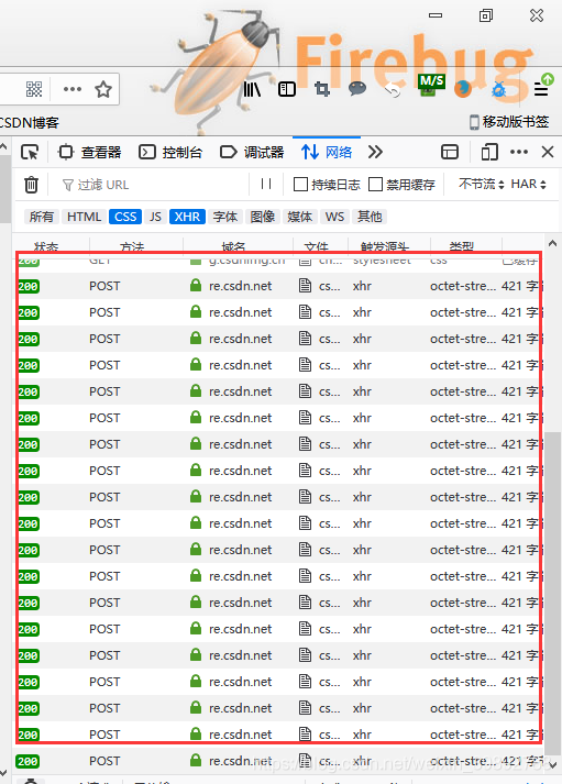
如图所示，如果不能复制User-Agent，点击 原始头；

如何为MATLAB配置ndbc的 HTTPS servers的证书（Certificate）？

% 本网页上面出现的一个标题：How can I configure MATLAB to allow access to self-signed HTTPS servers?
% 看Chirag Patel，2017-3-9这个人的回答；

Go to Google Chrome: Access same URL: Download Certificate (call it ndbc.cer)

Open Google Chrome. Click on Three Dots on Right-Top Most Corner, Select More Tools/Developer Tools –> Go to Security Tab –> Select View Certificate –> Go to Details Tab –> Click on Copy to File.
Download importcert.m ：

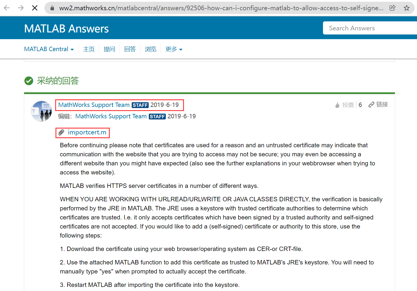
我是在https://ww2.mathworks.cn/matlabcentral/answers/92506-how-can-i-configure-matlab-to-allow-access-to-self-signed-https-servers下载的此文件：

function importcert(filename)
    if (nargin == 0)
        % If no certificate specified show open file dialog to select
        [filename,path] = uigetfile({'*.cer;*.crt','Certificates (*.cer,*.crt)'},'Select Certificate');
        if (filename==0), return, end
        filename = fullfile(path,filename);
    end
    % Determine Java keytool location and cacerts location
    keytool = fullfile(matlabroot,'sys','java','jre',computer('arch'),'jre','bin','keytool');
    cacerts = fullfile(matlabroot,'sys','java','jre',computer('arch'),'jre','lib','security','cacerts');
    % Create backup of cacerts
    if (~exist([cacerts '.org'],'file'))
        copyfile(cacerts,[cacerts '.org'])
    end
    % Construct and execute keytool
    command = sprintf('"%s" -import -file "%s" -keystore "%s" -storepass changeit',keytool,filename,cacerts);
    dos(command);

execute >> importcert('ndbc.cer')

执行时还要输入 yes，y，是…

具体忘记是哪一个了，好像是 y…

一个一个尝试吧~~
Restart MATLAB;

一定要重启！

matlab 如何储存大量数据比较合理？

https://www.zhihu.com/question/46755643

第一种是：用结构体实现，比如：a.b.c.d.e=matrix1

第二种是：用cell实现，但是可能必须（比如占用每一cell第一行）对数据对应属性进行描述。

题主是不是在纠结 cell 好还是 struct 好啊，我帮你再添加一个纠结的选项吧，你可以看看新出的 table 类型，这个可能比较适合你的需求

MATLAB如何使用table函数创建和编辑表格？

https://jingyan.baidu.com/article/f25ef254b9e3b5482d1b826a.html

table(列表1,列表2,列表3…)可以创建一个表格，其中的列表n可以是数值列向量，逻辑值列向量，categorical列向量，元胞数组列向量等等。

每个列表组成表格中的一列。
table函数可以带有参数’**VariableNames’**以指定列名称。

如图，指定第一列为Gender，第二列为Age，第三列为Vote。
table函数可以带有参数**’RowNames’**以指示每一行的行名称。

如图，将姓名列表指定为行名称。
table函数只有这两个额外选项，但是它们可以同时使用。

如图，同时指定’**RowNames’和‘VariableNames’**参数。
创建表格的另一种办法，是首先使用无参数的table创建空表格，然后给空表格添加列变量。

如图，使用T.Name=strs1; 在列表T中创建列Name，并把列表strs1的内容赋值给该列。
给列表添加信息可以使用列表属性。

如图，通过T.Properties.VariableNames可以获取或设置列名称；

通过T.Properties.RowNames可以获取或设置行名称；

通过T.Properties.DimensionNames可以获取或设置维度名称。
table表格所支持的属性值很多，除了正文中提到的，还有Description,VariableDescriptions,VariableUnits,UserData

second, function, path_save

function [ndbc_station_info] = ndbc_station_info(str,path_save)
% author:
%    liu jin can, UPC

% revison history
%    2022-02-12 first verison.
%    2022-02-19 second, function, path_save.

%%
disp('-----------------------ndbc_station_info')
cd(path_save)

%%
if contains(str,'default')
    load ndbc_station_info.mat
    save(strcat(path_save,'ndbc_station_info'),'ndbc_station_info')
else
    %% webread 正常运行
    url1 = 'https://www.ndbc.noaa.gov/to_station.shtml';
    %url2 = 'http://www.ndbc.noaa.gov/to_station.shtml'; %http 和 https 的区别：https://www.zhihu.com/question/436800837
    %url3 = 'https://blog.csdn.net/';
    %url4 = 'https://www.ndbc.noaa.gov';
    %url5 = 'http://baidu.com';
  
    UserAgent = 'Mozilla/5.0 (Windows NT 10.0; Win64; x64; rv:97.0) Gecko/20100101 Firefox/97.0';%如何查看火狐浏览器的useragent：https://blog.csdn.net/weixin_39892788/article/details/89875983
    %UserAgent = 'Mozilla/5.0 (Windows NT 10.0; Win64; x64) AppleWebKit/537.36 (KHTML, like Gecko) Chrome/95.0.4638.69 Safari/537.36';
  
    %options = weboptions();
    %options = weboptions('UserAgent',UserAgent);
    options = weboptions('UserAgent',UserAgent,'Timeout',120); %针对自己的浏览器填写
    % ,'CertificateFilename',''
    %设置模拟浏览器：https://blog.csdn.net/qq_40845110/article/details/115215561
  
    station_list_pagesource = webread(url1,options); %读取station_list的网页源代码
    %webread 和 urlread 的功能一样，[Contents Status] = urlread('https://www.ndbc.noaa.gov/to_station.shtml');
  
    %-------------------------------------------------------------------
    %  ps1：webread运行失败，直接去网页复制源代码所有内容，简单粘贴赋值给一个变量是不能的，另外，对于大量网页也是不可行的；
    %  ps2：webread运行失败可能的报错：未建立与 "https://www.ndbc.noaa.gov/to_station.shtml" 的安全连接，因为 "schannel: failed to receive handshake, SSL/TLS connection failed"。请检查您的系统证书是否过期、丢失或无效。
    %       webread运行失败可能的报错：无法建立与 "www.ndbc.noaa.gov" 的安全连接。原因是 ""。请检查您的证书文件(D:\Program Files (x86)\MATLAB\R2017b\sys\certificates\ca\rootcerts.pem)中的证书是否已过期、丢失或无效。
    %       webread运行失败可能的报错：无法建立与 "https://www.ndbc.noaa.gov/to_station.shtml" 的安全连接。原因是 "schannel: failed to receive handshake, SSL/TLS connection failed"。可能服务器不接受 HTTPS 连接。
    %  ps3：本人遇到的情况，matlab 2020a webread运行失败， matlab 2017b 运行成功，但是第二天早上运行2017b又失败了；
    %                       matlab 2020a，导入证书后成功，但是过一会儿又失败了；
    %                       matlab 2020a，导入证书，关闭clash代理后，成功；（希望别过一会儿又失败了）
    %       不知道为什么 ndbc 总是时不时的在抽风，有时候网页登不上去，不知道是不是自己网络的问题；
    %-------------------------------------------------------------------
    disp('ndbc webread 能正常运行。');
    table_station = table; %table类型；
  
    %% Text Analytics Toolbox 提取所有浮标ID（需要下载 Text Analytics Toolbox，下载时也需要关闭clash代理）
    hT = htmlTree(station_list_pagesource); %解析网页源代码
    %-------------------------------------------------------------------
    %  ps1：help htmlTree，2020版本有提示：'htmlTree' 需要 Text Analytics Toolbox。
    %                      2017没有提示；
    %-------------------------------------------------------------------
  
    % 在浏览器的网页中，观察源代码，发现所有浮标ID都在 <a></a> 标签里，
    % 且标签中的 href 都有h"station_page.php?station=" 部分；
    A_label = findElement(hT,'a'); %获取页面中所有a标签；
    A_label_href = getAttribute(A_label,'href'); %获取所有a标签的href内容；
    A_label_needed = A_label(contains(A_label_href,'station_page.php?station=')); %获取包含浮标ID的所有a标签
    %A_label_needed(171)
    %extractHTMLText(A_label_needed(171))
    station_ID = extractHTMLText(A_label_needed); %获取所有浮标的ID；
  
  
    disp('Text Analytics Toolbox 提取所有浮标ID成功。');
    save(strcat(path_save,'station_ID'),'station_ID')
    table_station.station_ID = station_ID; %将浮标的ID保存到table_station的第一列；
  
    %% Text Analytics Toolbox 提取每个浮标经度、纬度，tic toc 30分钟?
    station_lon = [];
    station_lat = [];
    warning_station = [];
    for i=1:1:size(table_station,1)
        % table_station 与 A_label_needed 站点ID一一顺序对应，不对应，输出错误；
        if(table_station{i,1}==extractHTMLText(A_label_needed(i)))
            % 获取网页的b标签内容
            href = getAttribute(A_label_needed(i),'href'); %得到指定浮标的href
            url = 'https://www.ndbc.noaa.gov/'+ href;
            pagesource = webread(url,options); %html
          
            hT = htmlTree(pagesource); %htmlTree
            B_label = findElement(hT,'b'); %b label
            B_text = extractHTMLText(B_label); % b label text
          
            % 从b标签内容筛选出lat和lon
            text0 = B_text( contains(B_text,'°') & ...
                contains(B_text,'(') & ...
                contains(B_text,')') & ...
                contains(B_text,'"')); % str,contains,?   % 例如显示为 "30.517 N 152.127 E (30°31'2" N 152°7'38" E)"
            if size(text0,1)~=1
                warning(table_station{i,1}+'经纬度提取失败，text0的维度不为1,为'+num2str(size(text0,1))+'。（大于1时很可能报错。）');
                warning_station = [warning_station;{table_station{i,1}}]
                lat = nan;
                lon = nan;
            else
                text0 = char(text0); %单引号 char, 双引号 string ：https://blog.csdn.net/weixin_43793141/article/details/105084788
                temp = strfind(text0,' '); %text 中空格的位置
                lat = text0(1:temp(1)+1); % char索引得到lat字符串
                lon = text0(temp(2)+1:temp(3)+1);
                disp('Text Analytics Toolbox 提取'+table_station{i,1}+'浮标经度、纬度成功。'+'i='+num2str(i));
            end
            % 加到station_lon，station_lat
            station_lat = [station_lat;{lat}]; % 以cell形式存储，加了{}
            station_lon = [station_lon;{lon}];
          
          
        else
            error('Text Analytics Toolbox 提取'+table_station{i,1}+'浮标经度、纬度时出错。');
        end
    end
  
    disp('Text Analytics Toolbox 提取每个浮标经度、纬度完成。');
    %save station_lat station_lat
    save(strcat(path_save,'station_lat'),'station_lat')
    save(strcat(path_save,'station_lon'),'station_lon')
    %save station_lon station_lon
    table_station.station_lat = station_lat;
    table_station.station_lon = station_lon;
  
    %% Text Analytics Toolbox 提取 Standard Meterological 历史数据年份信息
    station_historyYear = [];
    warning_station = [];
    url = 'https://www.ndbc.noaa.gov/historical_data.shtml';
    pagesource = webread(url,options);
    hT = htmlTree(pagesource); %htmlTree
    LI_label = findElement(hT,'li'); % li label, LI_label(13)
    LI_label_needed = LI_label(13); % 包含 Standard Meterological 的li label
    A_label = findElement(LI_label_needed,'a'); %a label
    A_label_href = getAttribute(A_label,'href'); %获取所有a标签的href内容；
  
    for i=1:1:size(table_station,1)
        temp = strcat('/download_data.php?filename=',lower(table_station{i,1}));%选择标准
        A_label_needed = A_label(contains(A_label_href,temp));
        if size(A_label_needed,1)>0
            historyYear = [extractHTMLText(A_label_needed)'];
            disp('Text Analytics Toolbox 提取'+table_station{i,1}+'的 Standard Meterological 历史数据年份信息成功。'+'i='+num2str(i));
        else
            warning(table_station{i,1}+'的 Standard Meterological 历史数据年份信息提取失败，historyYear的维度不大于0,为'+num2str(size(A_label_needed,1))+'。');
            warning_station = [warning_station;{table_station{i,1}}]
            historyYear = nan;
        end
        station_historyYear = [station_historyYear;{historyYear}];
    end
  
    disp('Text Analytics Toolbox 提取 Standard Meterological 历史数据年份信息完成。');
    %save station_historyYear station_historyYear
    save(strcat(path_save,'station_historyYear'),'station_historyYear')
    table_station.station__historyYear_SM = station_historyYear;
  
    %% ndbc_station_info
    ndbc_station_info = table_station;
    %save ndbc_station_info ndbc_station_info
    save(strcat(path_save,'ndbc_station_info'),'ndbc_station_info')
end

end

ndbc_station_info_needed.m

加载 ndbc_station_info.mat，创建包含所需NDBC浮标（or station）经纬度信息、所需数据年份信息的 ndbc_station_info_needed变量，保存到 ndbc_station_info_needed.mat。

ndbc_station_info_needed.m：

% author:
%    liu jin can, UPC

% revison history
%    2022-02-13 first verison.

clc, clear all
load ndbc_station_info.mat
disp('已加载ndbc_station_info.mat！'); pause(1);

%% 区域，needed
% 从gridgen.east-USA_P25.nml得到的经纬度范围
lat_max = 46;  % 纬度为负数，表示南纬
lat_min = 36;
lon_max = -58; % 经度为负数，表示西经
lon_min = -75;

% 将ndbc_station_info中的经纬度字符串信息转为数字，
% 例如
% '17.984 S'转换为-17.984
% '17.984 W'转换为-17.984
% cell类型的NaN转为数值的NaN
lat = [];
lon = [];
for i=1:1:size(ndbc_station_info,1)
    temp = cell2mat(ndbc_station_info{i,2}); %判断是否为nan
    if isnan(temp)
        lat = [lat;nan];
        lon = [lon;nan];
    else
        temp = char(ndbc_station_info{i,2}); %lat
        if temp(end)=='N'
            lat = [lat;str2num(temp(1:end-2))];
        elseif temp(end)=='S'
            lat = [lat;-str2num(temp(1:end-2))];
        end
      
        temp = char(ndbc_station_info{i,3}); %lon
        if temp(end)=='E'
            lon = [lon;str2num(temp(1:end-2))];
        elseif temp(end)=='W'
            lon = [lon;-str2num(temp(1:end-2))];
        end
    end
end

disp('已将ndbc_station_info中的经纬度字符串信息转为数字！'); pause(1);
ndbc_station_info.lat = lat;
ndbc_station_info.lon = lon;


% 选取所需区域的浮标
temp = find( ndbc_station_info.lat>=lat_min & ...
    ndbc_station_info.lat<=lat_max & ...
    ndbc_station_info.lon<=lon_max & ...
    ndbc_station_info.lon>=lon_min);
ndbc_station_info_needed0 = ndbc_station_info(temp,:);
disp('已将所需区域的浮标选取出来！'); pause(1);

%% 年份，needed
% 将所需区域浮标SM历史年份数据为nan的去除；
%ndbc_station_info_needed0.station__historyYear_SM{34}
temp = [];
for i=1:1:size(ndbc_station_info_needed0,1)
    try
        if isnan(ndbc_station_info_needed0.station__historyYear_SM{i})
            temp = [temp;0]; % nan 数据
        else
            temp = [temp;1]; % 单个字符串
        end
    catch
        temp = [temp;1]; % 多个字符串组成的string类型
    end
end
ndbc_station_info_needed0 = ndbc_station_info_needed0(logical(temp),:); %int8

%?特定年份？年份范围？
disp('已将所需区域对应年份的浮标选取出来！');pause(1);


%% save，在运行完前面的内容后，单独运行保存这一部分
%不支持将 'ndbc_station_info_needed' 同时用作变量名称和脚本名称。
%ndbc_station_info_needed = ndbc_station_info_needed0; 
%save ndbc_station_info_needed ndbc_station_info_needed

ndbc_station_info_needed变量：

second, function, path_save

function [ndbc_station_info_needed] = ndbc_station_info_needed(ndbc_station_info,lat_max,lat_min,lon_max,lon_min,path_save)
% author:
%    liu jin can, UPC

% revison history
%    2022-02-13 first verison.
%    2022-02-19 second, function, path_save.

%clc, clear all
%load ndbc_station_info.mat
%disp('已加载ndbc_station_info.mat！'); pause(1);

%%
disp('-----------------------ndbc_station_info_needed')
cd(path_save)

%% 区域，needed
% 从gridgen.east-USA_P25.nml得到的经纬度范围
%lat_max = 46;  % 纬度为负数，表示南纬
%lat_min = 36;
%lon_max = -58; % 经度为负数，表示西经
%lon_min = -75;

% 将ndbc_station_info中的经纬度字符串信息转为数字，
% 例如
% '17.984 S'转换为-17.984
% '17.984 W'转换为-17.984
% cell类型的NaN转为数值的NaN
lat = [];
lon = [];
for i=1:1:size(ndbc_station_info,1)
    temp = cell2mat(ndbc_station_info{i,2}); %判断是否为nan
    if isnan(temp)
        lat = [lat;nan];
        lon = [lon;nan];
    else
        temp = char(ndbc_station_info{i,2}); %lat
        if temp(end)=='N'
            lat = [lat;str2num(temp(1:end-2))];
        elseif temp(end)=='S'
            lat = [lat;-str2num(temp(1:end-2))];
        end
      
        temp = char(ndbc_station_info{i,3}); %lon
        if temp(end)=='E'
            lon = [lon;str2num(temp(1:end-2))];
        elseif temp(end)=='W'
            lon = [lon;-str2num(temp(1:end-2))];
        end
    end
end

disp('已将ndbc_station_info中的经纬度字符串信息转为数字！'); pause(1);
ndbc_station_info.lat = lat;
ndbc_station_info.lon = lon;


% 选取所需区域的浮标
temp = find( ndbc_station_info.lat>=lat_min & ...
    ndbc_station_info.lat<=lat_max & ...
    ndbc_station_info.lon<=lon_max & ...
    ndbc_station_info.lon>=lon_min);
ndbc_station_info_needed0 = ndbc_station_info(temp,:);
disp('已将所需区域的浮标选取出来！'); pause(1);

%% 年份，needed
% 将所需区域浮标SM历史年份数据为nan的去除；
%ndbc_station_info_needed0.station__historyYear_SM{34}
temp = [];
for i=1:1:size(ndbc_station_info_needed0,1)
    try
        if isnan(ndbc_station_info_needed0.station__historyYear_SM{i})
            temp = [temp;0]; % nan 数据
        else
            temp = [temp;1]; % 单个字符串
        end
    catch
        temp = [temp;1]; % 多个字符串组成的string类型
    end
end
ndbc_station_info_needed0 = ndbc_station_info_needed0(logical(temp),:); %int8

%?特定年份？年份范围？
disp('已将所需区域对应年份的浮标选取出来！');pause(1);


%% save，在运行完前面的内容后，单独运行保存这一部分
%不支持将 'ndbc_station_info_needed' 同时用作变量名称和脚本名称。
ndbc_station_info_needed = ndbc_station_info_needed0; 
%save ndbc_station_info_needed ndbc_station_info_needed
save(strcat(path_save,'ndbc_station_info_needed'),'ndbc_station_info_needed')

end

ndbc_station_info_needed_plot.m

加载 ndbc_station_info_needed.mat，用matlab中的m_map工具包对ndbc浮标进行绘图。

m_map工具包下载后是一个 m_map文件夹，调用时，需要添加 path(path,'m_map')，当然也可以将这个文件夹添加到matlab的环境中。

m_map工具包百度网盘：

链接：https://pan.baidu.com/s/1d2HEilJMh1XLItnuI3pVCw
提取码：mr76

ndbc_station_info_needed_plot.m：

% author:
%    liu jin can, UPC
%
% revison history
%    2022-02-13 first verison.
%    2022-02-18 second, 添加map到ndbc_station_download_NC_analyse;
%
% ps：许多 m_* 函数的应用，可以在 https://www.eoas.ubc.ca/~rich/map.html 网页，crtl+F搜索使用其的例子。

clc, clear all
load ndbc_station_info_needed.mat
disp('已加载ndbc_station_info_needed.mat！'); pause(1);

%% 可调参数
% 区域范围信息
lon1 = -75; %100
lon2 = -58; %125
lat1 = 36; %0
lat2 = 46; %30

% 经度和纬度显示的刻度信息
xtick_lon = lon1:5:lon2;%
xticklabels_lon = num2str(xtick_lon');%
ytick_lat = lat1:2:lat2;
yticklabels_lat = num2str(ytick_lat');

% 水深colorbar信息
water_min = -6000; %水深范围；（先用jet去试试，确定后再用blue，因为blue中的白色容易漏掉，有特别深的水深数据）
etopo2_contourf = [water_min:-water_min/100:0]; % /10，/100，分母越大好像越好
CM_piece_num = 80;%colorbar平均分的块数
CM_type = 'blue'; % jet, gland
                  % CM_type 可以组合：CM = colormap([m_colmap('jet',CM_piece_num);m_colmap('gland',48)]); 
                  %                 自己去对应位置调；
CM_Ytick = fliplr([0 -1200  -2400 -3600 -4800 -6000]);  %colorbar刻度信息
CM_position = [0.8 0.1 0.0288 0.8]; %colorbar位置
CM_TickLength = [0.01 10]; %colorbar刻度长
             


% 浮标点的信息
point_lon = ndbc_station_info_needed.lon; %[108 116 119 114 116 110]';
point_lat = ndbc_station_info_needed.lat; %[20 21 20 17 11 14]';
% point_name=['P1', 'P2', 'P3', 'P4', 'P5'];
%point_name={'P1', 'P2', 'P3', 'P4', 'P5', 'P6'};
%buoy_name={'1','2','3','4','5','6','7','8','9'};


%% m_map
F1 = figure(1);
path(path,'m_map');

% m_proj：投影
m_proj('Mercator','lon',[lon1 lon2],'lat',[lat1 lat2]);%%矩形

% m_etopo2, m_contfbar：水深数据及其 colorbar
[CS,CH] = m_etopo2('contourf',etopo2_contourf,'edgecolor','none');
[ax,h] = m_contfbar(0.9,[0.2,0.8],CS,CH,'endpiece','no','axfrac',.05,'edgecolor','none',...
    'fontname','times new roman','fontsize',14);

% m_plot, m_text ：画点及标出名称
hold on
for ii=1:size(point_lon,1)
    m_plot(point_lon(ii),point_lat(ii),'ro','MarkerEdgeColor','r','MarkerFaceColor','r','markersize',5.2);
    hold on
    m_text(point_lon(ii),point_lat(ii),num2str(ii),'fontname','times new roman','FontSize',9);
    hold on
end




% m_gshhs_*：海岸线数据
%m_coast('patch',[.6 .6 .7]);
% m_gshhs_c('patch',[.7 .7 .7]);
%m_gshhs_l('patch',[.5 .5 .5]);
m_gshhs_i('patch',[.7 .7 .7]);
%m_gshhs_f('patch',[.7 .7 .7]); %full


% m_grid：网格
m_grid('box','fancy','tickdir','in','tickstyle','dm','xtick',xtick_lon,...
    'xticklabels',xticklabels_lon,'ytick',ytick_lat,...
    'yticklabels',yticklabels_lat,'fontname','times new roman','FontSize',14,...
    'linestyle','none');
XL1 = xlabel('Longitude(°E)','fontsize',14,'fontname','Times New Roman');
YL1 = ylabel('Latitude(°N)','fontsize',14,'fontname','Times New Roman');

%% colorbar的设置
% figure 背景为白色
set(gcf,'color','w');  % otherwise 'print' turns lakes black

% 水深colorbar信息
CM = colormap(m_colmap(CM_type,CM_piece_num));
% CM = colormap([m_colmap('jet',CM_piece_num);m_colmap('gland',48)]); %colormap选取

set(ax.YLabel,'string','Water Depth (m)','fontname','times new roman','fontsize',14'); %colorbar对应的名称
set(ax,'position',CM_position,...
    'Ytick',CM_Ytick,...%'Yticklabel',{'0';'600';'1200';'1800';'2400';'3000';'3600';'4200';'4800';'5400';'6000'},...
    'YTickLabelMode','auto',...
    'TickLength',CM_TickLength,...
    'Ydir','reverse'); %colorbar位置，刻度


%% 添加map到ndbc_station_download_NC_analyse
%load ndbc_station_download_NC_analyse
%savefig(F1,strcat('.\fig\区域ndbc浮标图','.fig'));
%ndbc_station_download_NC_analyse.BuoyPointsMap{1,1} = strcat('openfig(".\fig\区域ndbc浮标图','.fig")');
%close(F1)
%save ndbc_station_download_NC_analyse ndbc_station_download_NC_analyse

运行得到的图形（还需要调整参数才能更好看，这里就粗略咯）：

可以根据标号确定索引，选择想要点的浮标；

南海论文中浮标的图

Step0_plot_quyu_buoy.m：

%%%%画图
clc,clear all

%% 参数
while(1)
    lon1=100;
    lon2=125;
    lat1=0;
    lat2=30;
  
    point_lon=[108 116 119 114 116 110]';
    point_lat=[20 21 20 17 11 14]';
    % point_name=['P1', 'P2', 'P3', 'P4', 'P5'];
    point_name={'P1', 'P2', 'P3', 'P4', 'P5', 'P6'};
    buoy_name={'1','2','3','4','5','6','7','8','9'};
    break
end

%% 句柄
while(1)
    F1 = figure(1);
    path(path,'m_map');
    m_proj('Mercator','lon',[lon1 lon2],'lat',[lat1 lat2]);%%矩形
    %
    [CS,CH]=m_etopo2('contourf',[-6000:200:0],'edgecolor','none');
    [ax,h]=m_contfbar(0.9,[0.2,0.8],CS,CH,'endpiece','no','axfrac',.05,'edgecolor','none',...
        'fontname','times new roman','fontsize',14);
  
    hold on
    for ii=1:5
        m_plot(point_lon(ii),point_lat(ii),'ro','MarkerEdgeColor','r','MarkerFaceColor','r','markersize',5.2);
        hold on
        % m_text(point_lon(ii)-0.3,point_lat(ii)-0.6,point_name(2*(ii-1)+1:2*(ii-1)+2),'fontsize',12)
        point_name{ii};
        m_text(point_lon(ii)-0.7,point_lat(ii)-0.9,point_name{ii},'fontname','times new roman','FontSize',9);
        hold on
    end
  
    m_plot(point_lon(6),point_lat(6),'ro','MarkerEdgeColor','r','MarkerFaceColor','r','markersize',5.2);
    hold on
    point_name{6};
    m_text(point_lon(6)-0.5,point_lat(6)-0.9,point_name{6},'fontname','times new roman','FontSize',9);
    hold on
  
    %m_coast('patch',[.6 .6 .7]);
    % m_gshhs_c('patch',[.7 .7 .7]);
    %m_gshhs_l('patch',[.5 .5 .5]);
    m_gshhs_i('patch',[.7 .7 .7]);
    %m_gshhs_f('patch',[.7 .7 .7]); %full
  
    m_grid('box','fancy','tickdir','in','tickstyle','dm','xtick',[100 105 110 115 120 125 130 135],...
        'xticklabels',['100';'105';'110';'115';'120';'125';'130';'135';],'ytick',[5 10 15 20 25 30 35 40],...
        'yticklabels',['5 '; '10';'15';'20';'25';'30';'35';'40'],'fontname','times new roman','FontSize',14,...
        'linestyle','none');
    XL1 = xlabel('Longitude(°E)','fontsize',14,'fontname','Times New Roman');
    YL1 = ylabel('Latitude(°N)','fontsize',14,'fontname','Times New Roman');
    %
    A=[105 105 120 120 105;9 25 25 9 9];
    m_plot(A(1,:),A(2,:),'r-','linewidth',2);
  
    %
    point_lon=[118.2  116.17 117.34 119 111.53 111.83  111 117.29 109.17]';
    point_lat=[23.63 22.15  22.33  22.6 20.73 19.35 18.51 20.99 20.5]';
    hold on
    try
        m_plot(point_lon(1),point_lat(1),'s','MarkerEdgeColor','k','MarkerFaceColor','k','markersize',4);hold on %右移--加。下移--减。
        m_text(point_lon(1)+0.4,point_lat(1)+0.1,buoy_name{1},'fontname','times new roman','FontSize',8);hold on %左移--减。上移--加。

        m_plot(point_lon(2),point_lat(2),'s','MarkerEdgeColor','k','MarkerFaceColor','k','markersize',4);hold on %右移--加。下移--减。
        m_text(point_lon(2)-0.8,point_lat(2)+0.1,buoy_name{2},'fontname','times new roman','FontSize',8);hold on %左移--减。上移--加。
      
        m_plot(point_lon(3),point_lat(3),'s','MarkerEdgeColor','k','MarkerFaceColor','k','markersize',4);hold on %右移--加。下移--减。
        m_text(point_lon(3)+0.4,point_lat(3)+0.1,buoy_name{3},'fontname','times new roman','FontSize',8);hold on %左移--减。上移--加。
      
        m_plot(point_lon(4),point_lat(4),'s','MarkerEdgeColor','k','MarkerFaceColor','k','markersize',4);hold on %右移--加。下移--减。
        m_text(point_lon(4)+0.4,point_lat(4)+0.1,buoy_name{4},'fontname','times new roman','FontSize',8);hold on %左移--减。上移--加。
      
        m_plot(point_lon(5),point_lat(5),'s','MarkerEdgeColor','k','MarkerFaceColor','k','markersize',4);hold on %右移--加。下移--减。
        m_text(point_lon(5)+0.4,point_lat(5)+0.1,buoy_name{5},'fontname','times new roman','FontSize',8);hold on %左移--减。上移--加。
      
        m_plot(point_lon(6),point_lat(6),'s','MarkerEdgeColor','k','MarkerFaceColor','k','markersize',4);hold on %右移--加。下移--减。
        m_text(point_lon(6)+0.4,point_lat(6)+0.1,buoy_name{6},'fontname','times new roman','FontSize',8);hold on %左移--减。上移--加。
      
        m_plot(point_lon(7),point_lat(7),'s','MarkerEdgeColor','k','MarkerFaceColor','k','markersize',4);hold on %右移--加。下移--减。
        m_text(point_lon(7)+0.4,point_lat(7)+0.1,buoy_name{7},'fontname','times new roman','FontSize',8);hold on %左移--减。上移--加。
      
        m_plot(point_lon(8),point_lat(8),'s','MarkerEdgeColor','k','MarkerFaceColor','k','markersize',4);hold on %右移--加。下移--减。
        m_text(point_lon(8)+0.4,point_lat(8)+0.1,buoy_name{8},'fontname','times new roman','FontSize',8);hold on %左移--减。上移--加。
      
        m_plot(point_lon(9),point_lat(9),'s','MarkerEdgeColor','k','MarkerFaceColor','k','markersize',4);hold on %右移--加。下移--减。
        m_text(point_lon(9)-0.8,point_lat(9)+0.1,buoy_name{9},'fontname','times new roman','FontSize',8);hold on %左移--减。上移--加。
    end
    break
end

%% 调参
while(1)
    %----------------------------------------%
    CM_piece_num = 10;%colorbar
    CM = colormap(m_colmap('blues',CM_piece_num));%colormap(jet(CM_piece_num)); %colormap(m_colmap('blues')); %CM = colormap(cool(CM_piece_num));
    %cmocean_deep;% cmocean__deep; % colormap(cmocean__deep(round((256/5)*(1:1:5)),:));
  
    set(gcf,'color','w');  % otherwise 'print' turns lakes black
    set(ax.YLabel,'string','Water Depth (m)','fontname','times new roman','fontsize',14');
    set(ax,'position',[0.8 0.1 0.0388 0.8],...
        'Ytick',fliplr([0 -1200  -2400 -3600 -4800 -6000]),...%'Yticklabel',{'0';'600';'1200';'1800';'2400';'3000';'3600';'4200';'4800';'5400';'6000'},...
        'YTickLabelMode','auto',...
        'TickLength',[0.01 0.01],...
        'Ydir','reverse');
      

    break
end

运行结果：

second, function, path_save

function [ndbc_station_info_needed] = ndbc_station_info_needed_plot(ndbc_station_info_needed,lat_max,lat_min,lon_max,lon_min,path_save)
% author:
%    liu jin can, UPC
%
% revison history
%    2022-02-13 first verison.
%    2022-02-19 second, function, path_save.
%
% ps：许多 m_* 函数的应用，可以在 https://www.eoas.ubc.ca/~rich/map.html 网页，crtl+F搜索使用其的例子。

%clc, clear all
%load ndbc_station_info_needed.mat
%disp('已加载ndbc_station_info_needed.mat！'); pause(1);

%%
disp('-----------------------ndbc_station_info_needed_plot')
cd(path_save)

%% 可调参数
% 区域范围信息
lon1 = lon_min; %100
lon2 = lon_max; %125
lat1 = lat_min; %0
lat2 = lat_max; %30

% 经度和纬度显示的刻度信息
xtick_lon = lon1:5:lon2;%
xticklabels_lon = num2str(xtick_lon');%
ytick_lat = lat1:2:lat2;
yticklabels_lat = num2str(ytick_lat');

% 水深colorbar信息
water_min = -6000; %水深范围；（先用jet去试试，确定后再用blue，因为blue中的白色容易漏掉，有特别深的水深数据）
etopo2_contourf = [water_min:-water_min/100:0]; % /10，/100，分母越大好像越好
CM_piece_num = 80;%colorbar平均分的块数
CM_type = 'blue'; % jet, gland
% CM_type 可以组合：CM = colormap([m_colmap('jet',CM_piece_num);m_colmap('gland',48)]);
%                 自己去对应位置调；
CM_Ytick = fliplr([0 -1200  -2400 -3600 -4800 -6000]);  %colorbar刻度信息
CM_position = [0.8 0.1 0.0288 0.8]; %colorbar位置
CM_TickLength = [0.01 10]; %colorbar刻度长



% 浮标点的信息
point_lon = ndbc_station_info_needed.lon; %[108 116 119 114 116 110]';
point_lat = ndbc_station_info_needed.lat; %[20 21 20 17 11 14]';
% point_name=['P1', 'P2', 'P3', 'P4', 'P5'];
%point_name={'P1', 'P2', 'P3', 'P4', 'P5', 'P6'};
%buoy_name={'1','2','3','4','5','6','7','8','9'};


%% m_map
F1 = figure(1);
% m_map
%cd(path_save);
%cd('..'); % 跳到上一级路径下
%path(path,'\m_map');
%cd(path_save) % 返回之前的路径


% m_proj：投影
m_proj('Mercator','lon',[lon1 lon2],'lat',[lat1 lat2]);%%矩形

% m_etopo2, m_contfbar：水深数据及其 colorbar
[CS,CH] = m_etopo2('contourf',etopo2_contourf,'edgecolor','none');
[ax,h] = m_contfbar(0.9,[0.2,0.8],CS,CH,'endpiece','no','axfrac',.05,'edgecolor','none',...
    'fontname','times new roman','fontsize',14);

% m_plot, m_text ：画点及标出名称
hold on
for ii=1:size(point_lon,1)
    m_plot(point_lon(ii),point_lat(ii),'ro','MarkerEdgeColor','r','MarkerFaceColor','r','markersize',5.2);
    hold on
    m_text(point_lon(ii),point_lat(ii),num2str(ii),'fontname','times new roman','FontSize',9);
    hold on
end




% m_gshhs_*：海岸线数据
%m_coast('patch',[.6 .6 .7]);
% m_gshhs_c('patch',[.7 .7 .7]);
%m_gshhs_l('patch',[.5 .5 .5]);
m_gshhs_i('patch',[.7 .7 .7]);
%m_gshhs_f('patch',[.7 .7 .7]); %full


% m_grid：网格
m_grid('box','fancy','tickdir','in','tickstyle','dm','xtick',xtick_lon,...
    'xticklabels',xticklabels_lon,'ytick',ytick_lat,...
    'yticklabels',yticklabels_lat,'fontname','times new roman','FontSize',14,...
    'linestyle','none');
XL1 = xlabel('Longitude(°E)','fontsize',14,'fontname','Times New Roman');
YL1 = ylabel('Latitude(°N)','fontsize',14,'fontname','Times New Roman');

%% colorbar的设置
% figure 背景为白色
set(gcf,'color','w');  % otherwise 'print' turns lakes black

% 水深colorbar信息
CM = colormap(m_colmap(CM_type,CM_piece_num));
% CM = colormap([m_colmap('jet',CM_piece_num);m_colmap('gland',48)]); %colormap选取

set(ax.YLabel,'string','Water Depth (m)','fontname','times new roman','fontsize',14'); %colorbar对应的名称
set(ax,'position',CM_position,...
    'Ytick',CM_Ytick,...%'Yticklabel',{'0';'600';'1200';'1800';'2400';'3000';'3600';'4200';'4800';'5400';'6000'},...
    'YTickLabelMode','auto',...
    'TickLength',CM_TickLength,...
    'Ydir','reverse'); %colorbar位置，刻度

%% 添加map到ndbc_station_download_NC_analyse
%load ndbc_station_download_NC_analyse
mkdir fig
savefig(F1,strcat(path_save,'fig\区域ndbc浮标图','.fig'));
ndbc_station_info_needed.BuoyPointsMap{1,1} = strcat('cd(path_save); openfig(".\fig\区域ndbc浮标图','.fig")');
%ndbc_station_download_NC_analyse.BuoyPointsMap{1,1} = strcat('openfig(".\fig\区域ndbc浮标图','.fig")');
close(F1)
%save ndbc_station_download_NC_analyse ndbc_station_download_NC_analyse
end

ndbc_station_info_needed_etopo1.m

加载 ndbc_station_info_needed.mat，获取对应浮标的 etopo1水深数据，etopo1.nc位于 m_map\ETOPO1\。

ndbc_station_info_needed_etopo1.m：

clc, clear all
load ndbc_station_info_needed.mat
disp('已加载ndbc_station_info_needed.mat！'); pause(1);

%%%%%%%%%%%  水深  %%%%%%%%%%%
lon = ncread('m_map\ETOPO1\etopo1.nc', 'lon');
lat = ncread('m_map\ETOPO1\etopo1.nc', 'lat');
water = ncread('m_map\ETOPO1\etopo1.nc', 'z');

%%%% 提取特定位置的水深 %%%%%
point_lon=[108 116 119 114 116 110]';
point_lat=[20 21 20 17 11 14]';
depth = zeros(1,length(point_lon));

for i = 1:1:length(point_lon)
    a = find(lat==point_lat(i));
    b = find(lon==point_lon(i));
    c = water(b,a);
  
    depth(i) = c;
end

second, function, path_save

function [ndbc_station_info_needed] = ndbc_station_info_needed_etopo1(ndbc_station_info_needed,path_save)
% author:
%    liu jin can, UPC

% revison history
%    2022-02-19 second verison, function, path_save.
%
% ps:
%    etopo1的经度范围是0~360
%    ndbc_station_info_needed的经度范围是-180~180

%clc, clear all
%load ndbc_station_info_needed.mat
%disp('已加载ndbc_station_info_needed.mat！'); pause(1);

disp('-----------------------ndbc_station_info_needed_etopo1')
%%%%%%%%%%%  水深  %%%%%%%%%%%
cd(path_save)
cd('..')
%ncdisp('m_map\ETOPO1\etopo1.nc')
lon = ncread('m_map\ETOPO1\etopo1.nc', 'lon');
lat = ncread('m_map\ETOPO1\etopo1.nc', 'lat');
water = ncread('m_map\ETOPO1\etopo1.nc', 'z');

%%%% 提取特定位置的水深 %%%%%
% 经度范围是-180~180，变成0~360
point_lon = ndbc_station_info_needed.lon;
tf = find(point_lon<0);
point_lon(tf) = point_lon(tf)+360;
%
point_lat = ndbc_station_info_needed.lat;
depth = zeros(length(point_lon),1);
% 查找每个浮标对应NC文件的最近网格点经纬度（索引）
for i=1:1:size(point_lon,1)
    % lat 最近网格点经纬度
    [~,a] = min(abs(lat(:)-point_lat(i))); 
    % lon 最近网格点经纬度
    [~,b] = min(abs(lon(:)-point_lon(i))); 
    % 
    c = water(b,a);
    depth(i) = c;
end

ndbc_station_info_needed.etopo1 = depth;

%% 可以去 https://www.ndbc.noaa.gov/to_station.shtml 查找一些浮标的水深，验证etopo1的准确性


end

etopo1来源机构及其论文参考

水深数据采用 NOAA 的地球物理数据中心(National Geophysical Data Center，NGDC)提供的 ETOPO-1 数据(Amante and Eakins,2009)。

ndbc_station_download.m

加载 ndbc_station_info_needed.mat，根据 ndbc_station_info_needed变量的信息，从网页上爬取对应所需数据矩阵，并以table数据形式存储浮标的数据矩阵（一个浮标、一个table），将所有浮标的table放在 ndbc_station_download变量，最终生成 ndbc_station_download.mat。

ps，保存成mat比txt所占内存更小。

存在bug，num2str()，暂时先放着~~

网页上的一个浮标一年的数据例子：

ndbc_station_download.m：

% author:
%    liu jin can, UPC
%
% revison history
%    2022-02-14 first verison. bug：num2str()

clc, clear all
load ndbc_station_info_needed.mat
disp('已加载ndbc_station_info_needed.mat！'); pause(1);
UserAgent = 'Mozilla/5.0 (Windows NT 10.0; Win64; x64; rv:97.0) Gecko/20100101 Firefox/97.0';%如何查看火狐浏览器的useragent：https://blog.csdn.net/weixin_39892788/article/details/89875983
options = weboptions('UserAgent',UserAgent,'Timeout',120); %针对自己的浏览器填写

%% 提取浮标的 Standard Meterological 历史数据
for i=[2 5 7]%1:1:size(ndbc_station_info_needed,1) %浮标循环
    disp('---------------------------------------------')
    % 确定存储浮标历史数据的数据结构：table
    buoy_table = table;
    buoy_table.YY{1,1} = [];
    buoy_table.MM{1,1} = [];
    buoy_table.DD{1,1} = [];
    buoy_table.hh{1,1} = [];
    buoy_table.mm{1,1} = [];
    buoy_table.WDIR{1,1} = [];
    buoy_table.WSPD{1,1} = [];
    buoy_table.GST{1,1} = [];
    buoy_table.WVHT{1,1} = [];
    buoy_table.DPD{1,1} = [];
    buoy_table.APD{1,1} = [];
    buoy_table.MWD{1,1} = [];
    buoy_table.PRES{1,1} = [];
    buoy_table.ATMP{1,1} = [];
    buoy_table.WTMP{1,1} = [];
    buoy_table.DEWP{1,1} = [];
    buoy_table.VIS{1,1} = [];
    buoy_table.TIDE{1,1} = [];
    buoy_table.Properties.VariableUnits = {'yr' 'mo' 'dy' 'hr' 'mn' 'degT' 'm/s' 'm/s' 'm' 'sec' 'sec' 'degT' 'hPa' 'degC' 'degC' 'degC' 'mi' 'ft'};
    buoy_table.Properties.VariableDescriptions = {'年' '月' '日' '小时' '分钟' 'degT' 'm/s' 'm/s' '有效波高' 'sec' 'sec' 'degT' 'hPa' 'degC' 'degC' 'degC' 'mi' 'ft'};
  
    % 记录导入失败的浮标
    buoy_fail = [];
  
    % 获取table中各项所需数据 18：YY  MM DD hh mm WDIR WSPD GST  WVHT   DPD   APD MWD   PRES  ATMP  WTMP  DEWP  VIS  TIDE
    count = 0; %输入数据进入table时,需要的索引；
    for j=1:1:size(ndbc_station_info_needed.station__historyYear_SM{i,1},2)%历史数据年份循环,[1 19]
        % 获取浮标某年的网页数据；
        %   % size(ndbc_station_info_needed.station__historyYear_SM{12,1},2)
        %   % size(ndbc_station_info_needed.station__historyYear_SM{17,1},2)
        temp = ndbc_station_info_needed.station__historyYear_SM{i,1};
        nian = temp{1,j};
        url = 'https://www.ndbc.noaa.gov/view_text_file.php?filename='+...
            lower(ndbc_station_info_needed{i,1})+'h'+...
            nian+'.txt.gz&dir=data/historical/stdmet/';
        %url = 'https://www.ndbc.noaa.gov/view_text_file.php?filename=41002h1976.txt.gz&dir=data/historical/stdmet/';
        pagesource = webread(url,options); %pagesource(1:100)
        %temp=find(isstrprop(pagesource(1:200),'digit')==1);pagesource(1:temp(1));
      
        % 获取 pagesource 第一次出现数字的索引，从而通过str2num()得到数据矩阵
        temp = find(isstrprop(pagesource(1:200),'digit')==1); %数据中出现数字的索引；
        [data,tf]= str2num(pagesource(temp(1):end)); %网页上得到的一年的数据，后面会对其列数进行验证。
        %[data,tf]= str2num(pagesource(temp(1):166));  %1
        %[data,tf]= str2num(pagesource(temp(1):167));  %0
        %[data,tf]= str2num(pagesource(temp(1):246)); %1
        %  上面tf的变化，说明当第一行数据的列数确定后，猜测通过/enter换行？，后面的数据列数如果存在缺失，返回[]；
        %  上面的规则基本保证使用str2num()是没大问题的！
      
      
        % 判别网页数据格式是在哪一时间段，从而知道每一列代表什么；
        % ndbc 数据不同年份的数据格式：
        %          1970-1998，索引~79，16列，YY MM DD hh WD   WSPD GST  WVHT  DPD   APD  MWD  BAR    ATMP  WTMP  DEWP  VIS
        %          1999，索引~81，16列，YYYY MM DD hh WD   WSPD GST  WVHT  DPD   APD  MWD  BAR    ATMP  WTMP  DEWP  VIS
        %          2000-2004，索引~87，17列，YYYY MM DD hh WD   WSPD GST  WVHT  DPD   APD  MWD  BAR    ATMP  WTMP  DEWP  VIS  TIDE
        %          2005-2006，索引~90，18列，YYYY MM DD hh mm  WD  WSPD GST  WVHT  DPD   APD  MWD  BAR    ATMP  WTMP  DEWP  VIS  TIDE
        %          2007-2020，索引179>150，18列，#YY  MM DD hh mm WDIR WSPD GST  WVHT   DPD   APD MWD   PRES  ATMP  WTMP  DEWP  VIS  TIDE
        %                              #yr  mo dy hr mn degT m/s  m/s     m   sec   sec degT   hPa  degC  degC  degC   mi    ft
      
      
        if(size(data,2)==16 & pagesource(3)== ' ') %1970-1998
            % YY+1900 MM DD hh （mm=0） WD   WSPD GST  WVHT  DPD   APD MWD  BAR    ATMP  WTMP  DEWP  VIS (TIDE)
            % data 的改造
            data = [data(:,1)+1900 data(:,2:4) zeros(size(data,1),1) data(:,5:16) 99*ones(size(data,1),1)];
            % 导入 data 进入 table
            buoy_table{count+1:count+size(data,1),1:18} = num2cell(data);
            count = count+size(data,1);
            disp('已导入'+lower(ndbc_station_info_needed{i,1})+'h'+nian+'数据到对应浮标的table！');
        elseif(size(data,2)==16 & pagesource(3)== 'Y') %1999
            % data 的改造
            data = [data(:,1) data(:,2:4) zeros(size(data,1),1) data(:,5:16) 99*ones(size(data,1),1)];
            buoy_table{count+1:count+size(data,1),1:18} = num2cell(data);
            count = count+size(data,1);
            disp('已导入'+lower(ndbc_station_info_needed{i,1})+'h'+nian+'数据到对应浮标的table！');
        elseif(size(data,2)==17) %2000-2004
            % data 的改造
            data = [data(:,1) data(:,2:4) zeros(size(data,1),1) data(:,5:17)];
            buoy_table{count+1:count+size(data,1),1:18} = num2cell(data);
            count = count+size(data,1);
            disp('已导入'+lower(ndbc_station_info_needed{i,1})+'h'+nian+'数据到对应浮标的table！');
        elseif(size(data,2)==18) %2005-2020
            buoy_table{count+1:count+size(data,1),1:18} = num2cell(data);
            count = count+size(data,1);
            disp('已导入'+lower(ndbc_station_info_needed{i,1})+'h'+nian+'数据到对应浮标的table！');
        else
            warning(lower(ndbc_station_info_needed{i,1})+'h'+nian+'不符合一般的数据格式特点？i='+num2str(i)+',j='+num2str(j)+',tf='+num2str(tf)+',导入table失败。');
            warning('若tf=0，那么str2num()出现问题，导致data=[]，根本原因可能是TIDE数据有缺失空白。')
            buoy_fail = [buoy_fail;{lower(ndbc_station_info_needed{i,1})+'h'+nian+'不符合一般的数据格式特点？i='+num2str(i)+',j='+num2str(j)+',tf='+num2str(tf)+',导入table失败。'}];
            %44008h2000不符合一般的数据格式特点？i=5,j=19  %%TIDE 有空白
            %44008h2017不符合一般的数据格式特点？i=5,j=35
            %error(lower(ndbc_station_info_needed{i,1})+'h'+nian+'可能在调用str2num()时出错，因为矩阵列数不为16，不符合1970-1998的数据格式特点？。');
        end
      
      
    end
  
    % 存储浮标历史数据的table保存到： ndbc_station_info_needed.station_historyData_SM{i,1}
    ndbc_station_info_needed.station_historyData_SM{i,1} = buoy_table;
    ndbc_station_info_needed.station_historyData_SM{i,2} = buoy_fail;
    disp('已导入'+lower(ndbc_station_info_needed{i,1})+'的table数据到ndbc_station_info_needed.station_historyData_SM！');

end

disp('已提取浮标的 Standard Meterological 历史数据到 ndbc_station_info_needed。')

%% save
%ndbc_station_download = ndbc_station_info_needed;
%save ndbc_station_download ndbc_station_download

运行生成的 ndbc_station_download变量：（2、5、7浮标标号对应plot中的2、5、7标号，用这3个浮标进行数据分析）

问题得到大佬们的指点解决：str2num()

要求char中没有字母，否则返回[]；

数据缺失也会返回[]；

ndbc 数据不同年份的数据格式

EB01: 1970 1971 1972 1973 1974 1975 ；

https://www.ndbc.noaa.gov/historical_data.shtml 的Standard Meterological中，crtl+F搜索到最早的是 1970年；

41002: 1976 1977 1978 1979 1980 1981 1982 1983 1984 1985 1986 1987 1988 1989 1990 1991 1992 1993 1994 1995 1996 1997 1998 1999 2000 2001 2002 2003 2004 2005 2006 2007 2008 2010 2012 2013 2014 2015 2016 2017 2018 2019 2020；

41009: 2009 2011 2012 2013 2014 2015 2016 2017 2018 2019 2020;

YY MM DD hh WD   WSPD GST  WVHT  DPD   APD  MWD  BAR    ATMP  WTMP  DEWP  VIS
70 02 26 20 009 14.9 99.0 99.00 99.00 99.00 999 1012.0  00.0 999.0  00.0 99.0


YY MM DD hh WD   WSPD GST  WVHT  DPD   APD  MWD  BAR    ATMP  WTMP  DEWP  VIS
71 01 01 01 109 15.9 99.0 99.00 99.00 99.00 999 1000.0  12.6 999.0 999.0 99.0

YY MM DD hh WD   WSPD GST  WVHT  DPD   APD  MWD  BAR    ATMP  WTMP  DEWP  VIS
72 01 09 19 129 10.9 99.0 99.00 99.00 99.00 999 1020.0  15.6 999.0  15.6 99.0

YY MM DD hh WD   WSPD GST  WVHT  DPD   APD  MWD  BAR    ATMP  WTMP  DEWP  VIS
73 01 01 13 229 07.7 99.0 99.00 99.00 99.00 999 1020.0  17.6 999.0  17.6 99.0

YY MM DD hh WD   WSPD GST  WVHT  DPD   APD  MWD  BAR    ATMP  WTMP  DEWP  VIS
74 01 25 13 050 06.1 99.0 99.00 99.00 99.00 999 1023.0  16.3 999.0  15.0 99.0

YY MM DD hh WD   WSPD GST  WVHT  DPD   APD  MWD  BAR    ATMP  WTMP  DEWP  VIS
75 01 01 00 165 09.0 99.0 99.00 99.00 99.00 999 1023.5  16.0 999.0  10.6 99.0

YY MM DD hh WD   WSPD GST  WVHT  DPD   APD  MWD  BAR    ATMP  WTMP  DEWP  VIS
76 01 01 00 197 16.6 99.0 99.00 99.00 99.00 999 1008.3  22.3  23.2 999.0 99.0

YY MM DD hh WD   WSPD GST  WVHT  DPD   APD  MWD  BAR    ATMP  WTMP  DEWP  VIS
77 01 01 00 294 14.0 99.0 02.90 99.00 06.50 999 1005.8  19.2  21.6 999.0 99.0

YY MM DD hh WD   WSPD GST  WVHT  DPD   APD  MWD  BAR    ATMP  WTMP  DEWP  VIS
78 01 01 00 293 06.2 99.0 02.10 99.00 06.50 999 1017.8  19.9  21.4 999.0 99.0

YY MM DD hh WD   WSPD GST  WVHT  DPD   APD  MWD  BAR    ATMP  WTMP  DEWP  VIS
79 01 20 00 358 02.3 99.0 99.00 99.00 99.00 999 1022.9  13.0  20.6 999.0 99.0

YY MM DD hh WD   WSPD GST  WVHT  DPD   APD  MWD  BAR    ATMP  WTMP  DEWP  VIS
80 01 01 00 281 09.9 12.6 99.00 99.00 99.00 999 1008.6  18.1  22.2 999.0 99.0

YY MM DD hh WD   WSPD GST  WVHT  DPD   APD  MWD  BAR    ATMP  WTMP  DEWP  VIS
81 01 01 00 301 07.8 10.2 02.20 11.10 06.30 999 1009.9  16.4  22.1 999.0 99.0

YY MM DD hh WD   WSPD GST  WVHT  DPD   APD  MWD  BAR    ATMP  WTMP  DEWP  VIS
82 01 03 15 151 07.6 09.3 01.80 09.10 05.70 999 1026.1  19.1  23.5 999.0 99.0

YY MM DD hh WD   WSPD GST  WVHT  DPD   APD  MWD  BAR    ATMP  WTMP  DEWP  VIS
83 01 01 01 077 02.0 02.8 01.90 09.10 06.10 999 1022.8  21.4  22.0 999.0 99.0

YY MM DD hh WD   WSPD GST  WVHT  DPD   APD  MWD  BAR    ATMP  WTMP  DEWP  VIS
84 01 01 00 357 13.9 17.9 04.70 09.10 06.70 999 1024.2  15.4  22.2 999.0 99.0

YY MM DD hh WD   WSPD GST  WVHT  DPD   APD  MWD  BAR    ATMP  WTMP  DEWP  VIS
85 01 01 00 167 04.9 06.1 99.00 99.00 99.00 999 1026.0  23.0  24.5 999.0 99.0

YY MM DD hh WD   WSPD GST  WVHT  DPD   APD  MWD  BAR    ATMP  WTMP  DEWP  VIS
86 03 26 18 097 09.8 12.1 02.20 08.30 05.30 999 1028.3  19.9  20.8 999.0 99.0

YY MM DD hh WD   WSPD GST  WVHT  DPD   APD  MWD  BAR    ATMP  WTMP  DEWP  VIS
87 01 01 00 063 07.1 09.0 01.60 10.00 05.20 999 1022.3  15.7  23.5 999.0 99.0

YY MM DD hh WD   WSPD GST  WVHT  DPD   APD  MWD  BAR    ATMP  WTMP  DEWP  VIS
88 01 01 00 144 02.6 04.6 02.20 12.50 08.80 999 1034.4  15.6  21.1 999.0 99.0

YY MM DD hh WD   WSPD GST  WVHT  DPD   APD  MWD  BAR    ATMP  WTMP  DEWP  VIS
89 01 01 01 068 04.2 05.5 01.40 05.60 05.10 999 1020.6  21.4  23.6 999.0 99.0

YY MM DD hh WD   WSPD GST  WVHT  DPD   APD  MWD  BAR    ATMP  WTMP  DEWP  VIS
90 03 27 21 038 09.9 12.5 02.20 07.70 05.50 999 1021.3  17.1  21.9 999.0 99.0

YY MM DD hh WD   WSPD GST  WVHT  DPD   APD  MWD  BAR    ATMP  WTMP  DEWP  VIS
91 01 01 00 246 03.0 06.5 01.90 11.10 06.00 999 1023.3  21.3  22.8 999.0 99.0

YY MM DD hh WD   WSPD GST  WVHT  DPD   APD  MWD  BAR    ATMP  WTMP  DEWP  VIS
92 01 01 00 083 11.4 13.9 03.40 10.00 06.70 999 1023.8  18.9  22.4 999.0 99.0

YY MM DD hh WD   WSPD GST  WVHT  DPD   APD  MWD  BAR    ATMP  WTMP  DEWP  VIS
93 01 01 00 202 04.5 05.5 02.00 10.00 07.60 999 1021.4  21.2  21.9 999.0 99.0

YY MM DD hh WD   WSPD GST  WVHT  DPD   APD  MWD  BAR    ATMP  WTMP  DEWP  VIS
94 01 01 00 315 03.4 05.5 01.40 10.00 05.70 999 1029.2  13.4  20.4 999.0 99.0

YY MM DD hh WD   WSPD GST  WVHT  DPD   APD  MWD  BAR    ATMP  WTMP  DEWP  VIS
95 01 01 00 135 10.3 12.9 02.60 06.20 06.10 999 1023.8  19.9  22.2 999.0 99.0

YY MM DD hh WD   WSPD GST  WVHT  DPD   APD  MWD  BAR    ATMP  WTMP  DEWP  VIS
96 01 01 00 163  8.6  9.9 99.00 99.00 99.00 999 1012.4  18.1  19.8 999.0 99.0

YY MM DD hh WD   WSPD GST  WVHT  DPD   APD  MWD  BAR    ATMP  WTMP  DEWP  VIS
97 01 01 00 235  4.6  5.6  1.32  5.26  5.02 999 1018.9  20.7  20.6 999.0 99.0

YY MM DD hh WD   WSPD GST  WVHT  DPD   APD  MWD  BAR    ATMP  WTMP  DEWP  VIS
98 01 01 00 289 14.1 18.9  4.41 10.00  7.04 999 1018.8  14.0  21.4 999.0 99.0

YYYY MM DD hh WD   WSPD GST  WVHT  DPD   APD  MWD  BAR    ATMP  WTMP  DEWP  VIS
1999 01 01 00 999 99.0 99.0 99.00 99.00 99.00 999 9999.0 999.0 999.0 999.0 99.0

1999年开始，YY更换为YYYY。

YYYY MM DD hh WD   WSPD GST  WVHT  DPD   APD  MWD  BAR    ATMP  WTMP  DEWP  VIS  TIDE
2000 01 01 00 275  5.0  5.9  1.42  6.25  5.14 999 1020.6  19.9  21.5 999.0 99.0

2000年开始，新增了TIDE，其部分数据是空白的，其他数据是否也会空白？。

YYYY MM DD hh WD   WSPD GST  WVHT  DPD   APD  MWD  BAR    ATMP  WTMP  DEWP  VIS  TIDE
2001 01 01 00 280  8.1 11.2  2.01  7.14  5.29 999 1020.7  11.8  21.4 999.0 99.0 99.00

YYYY MM DD hh WD   WSPD GST  WVHT  DPD   APD  MWD  BAR    ATMP  WTMP  DEWP  VIS  TIDE
2002 01 01 00 129  8.1  9.6  0.72  7.69  5.64 999 1015.1  17.7  21.8 999.0 99.0 99.00

YYYY MM DD hh WD   WSPD GST  WVHT  DPD   APD  MWD  BAR    ATMP  WTMP  DEWP  VIS  TIDE
2003 01 01 00 168 10.7 12.9  2.05  7.14  5.39 999 1020.6  22.3  22.4  16.6 99.0 99.00

YYYY MM DD hh  WD  WSPD GST  WVHT  DPD   APD  MWD  BAR    ATMP  WTMP  DEWP  VIS  TIDE
2004 01 01 00  99  1.4  2.9  1.27  6.67  5.80 999 1026.8  19.0  23.0  10.5 99.0 99.00

YYYY MM DD hh mm  WD  WSPD GST  WVHT  DPD   APD  MWD  BAR    ATMP  WTMP  DEWP  VIS  TIDE
2005 01 01 00 00 177  3.1  4.0  0.93 10.00  6.43 999 1030.9  19.7  21.1  13.3 99.0 99.00

2005年开始，新增了mm。

YYYY MM DD hh mm  WD  WSPD GST  WVHT  DPD   APD  MWD  BAR    ATMP  WTMP  DEWP  VIS  TIDE
2006 01 01 00 00 225 11.4 13.5  1.85  6.25  4.79 999 9999.0  22.0  21.9 999.0 99.0 99.00

#YY  MM DD hh mm WDIR WSPD GST  WVHT   DPD   APD MWD   PRES  ATMP  WTMP  DEWP  VIS  TIDE
#yr  mo dy hr mn degT m/s  m/s     m   sec   sec degT   hPa  degC  degC  degC  nmi    ft
2007 01 01 00 00 119  8.0 10.4  1.25  8.33  5.19 999 1026.0  20.8  24.4  16.0 99.0 99.00

2007年开始，WD更换为WDIR，BAR更换为PRES，增添了单位这一行。

#YY  MM DD hh mm WDIR WSPD GST  WVHT   DPD   APD MWD   PRES  ATMP  WTMP  DEWP  VIS  TIDE
#yr  mo dy hr mn degT m/s  m/s     m   sec   sec deg    hPa  degC  degC  degC  nmi    ft
2008 01 01 00 00  58  3.7  5.1  1.77  6.25  5.57 999 1019.9  21.0  23.9 999.0 99.0 99.00

#YY  MM DD hh mm WDIR WSPD GST  WVHT   DPD   APD MWD   PRES  ATMP  WTMP  DEWP  VIS  TIDE
#yr  mo dy hr mn degT m/s  m/s     m   sec   sec degT   hPa  degC  degC  degC   mi    ft
2008 12 31 23 50 295  8.7 10.6  0.78  5.00  4.17 999 1016.4  22.2  24.1  14.9 99.0 99.00
2009 01 01 00 20 291 10.2 12.3  0.90  3.85  3.84 999 1016.6  22.1  24.1  14.8 99.0 99.00

可能出现这种虽然是2009年文件，但是有2008数据；

#YY  MM DD hh mm WDIR WSPD GST  WVHT   DPD   APD MWD   PRES  ATMP  WTMP  DEWP  VIS  TIDE
#yr  mo dy hr mn degT m/s  m/s     m   sec   sec deg    hPa  degC  degC  degC  nmi    ft
2010 04 19 03 50  39 10.3 13.0  2.47  9.09  5.32 999 1014.3  19.7  22.6  14.7 99.0 99.00

#YY  MM DD hh mm WDIR WSPD GST  WVHT   DPD   APD MWD   PRES  ATMP  WTMP  DEWP  VIS  TIDE
#yr  mo dy hr mn degT m/s  m/s     m   sec   sec degT   hPa  degC  degC  degC   mi    ft
2010 12 31 23 50 138  8.1  9.7  1.28  5.26  4.07 999 1022.5  21.9  22.3  14.6 99.0 99.00
2011 01 01 00 20 134  7.8  9.0  1.24  5.26  3.92 999 1022.8  22.0  22.3  14.7 99.0 99.00

#YY  MM DD hh mm WDIR WSPD GST  WVHT   DPD   APD MWD   PRES  ATMP  WTMP  DEWP  VIS  TIDE
#yr  mo dy hr mn degT m/s  m/s     m   sec   sec degT   hPa  degC  degC  degC   mi    ft
2011 12 31 23 50  67  2.2  2.8  0.38 10.00  5.15 999 1022.3  22.3  23.0  12.8 99.0 99.00
2012 01 01 00 20  82  2.3  2.9  0.40 10.00  5.37 999 1022.7  22.4  22.9  13.1 99.0 99.00

#YY  MM DD hh mm WDIR WSPD GST  WVHT   DPD   APD MWD   PRES  ATMP  WTMP  DEWP  VIS  TIDE
#yr  mo dy hr mn degT m/s  m/s     m   sec   sec degT   hPa  degC  degC  degC   mi    ft
2012 12 31 23 50 136  5.7  7.2  1.03  6.25  4.69  35 1024.5  21.0  22.4  13.5 99.0 99.00
2013 01 01 00 20 145  6.0  7.6 99.00 99.00 99.00 999 1024.4  21.1  22.4  13.1 99.0 99.00

#YY  MM DD hh mm WDIR WSPD GST  WVHT   DPD   APD MWD   PRES  ATMP  WTMP  DEWP  VIS  TIDE
#yr  mo dy hr mn degT m/s  m/s     m   sec   sec degT   hPa  degC  degC  degC   mi    ft
2013 12 31 23 50  37  6.2  7.8  1.11  5.26  4.84 336 1024.8  21.3  25.1  13.3 99.0 99.00
2014 01 01 00 20  47  6.0  8.2 99.00 99.00 99.00 999 1025.0  21.5  25.1  13.7 99.0 99.00

#YY  MM DD hh mm WDIR WSPD GST  WVHT   DPD   APD MWD   PRES  ATMP  WTMP  DEWP  VIS  TIDE
#yr  mo dy hr mn degT m/s  m/s     m   sec   sec degT   hPa  degC  degC  degC   mi    ft
2015 01 01 00 20  40  8.4 10.0 99.00 99.00 99.00 999 1023.8  21.4  24.1  16.9 99.0 99.00

#YY  MM DD hh mm WDIR WSPD GST  WVHT   DPD   APD MWD   PRES  ATMP  WTMP  DEWP  VIS  TIDE
#yr  mo dy hr mn degT m/s  m/s     m   sec   sec degT   hPa  degC  degC  degC   mi    ft
2015 12 31 23 50 153  3.0  3.7  0.90  8.33  5.54  96 1020.0  25.2  25.2  23.3 99.0 99.00
2016 01 01 00 20 161  2.6  3.1 99.00 99.00 99.00 999 1020.4  25.3  25.2  23.2 99.0 99.00

#YY  MM DD hh mm WDIR WSPD GST  WVHT   DPD   APD MWD   PRES  ATMP  WTMP  DEWP  VIS  TIDE
#yr  mo dy hr mn degT m/s  m/s     m   sec   sec degT   hPa  degC  degC  degC   mi    ft
2017 04 22 15 30 161  5.2  6.7 99.00 99.00 99.00 999 1016.2  24.4  24.0  19.9 99.0 99.00 

#YY  MM DD hh mm WDIR WSPD GST  WVHT   DPD   APD MWD   PRES  ATMP  WTMP  DEWP  VIS  TIDE
#yr  mo dy hr mn degT m/s  m/s     m   sec   sec degT   hPa  degC  degC  degC   mi    ft
2018 01 01 00 00 330  3.3  4.9 99.00 99.00 99.00 999 1020.3  18.0  24.3  13.6 99.0 99.00 

#YY  MM DD hh mm WDIR WSPD GST  WVHT   DPD   APD MWD   PRES  ATMP  WTMP  DEWP  VIS  TIDE
#yr  mo dy hr mn degT m/s  m/s     m   sec   sec degT   hPa  degC  degC  degC   mi    ft
2019 01 01 00 00 156  6.3  7.9 99.00 99.00 99.00 999 1021.7  24.3 999.0  21.7 99.0 99.00 

#YY  MM DD hh mm WDIR WSPD GST  WVHT   DPD   APD MWD   PRES  ATMP  WTMP  DEWP  VIS  TIDE
#yr  mo dy hr mn degT m/s  m/s     m   sec   sec degT   hPa  degC  degC  degC   mi    ft
2020 01 01 00 00 288  4.1  5.6 99.00 99.00 99.00 999 1017.9  18.5  25.0   8.1 99.0 99.00

ndbc_station_download.m（第二版本, 使用 datetime 数据类型）

% author:
%    liu jin can, UPC
%
% revison history
%    2022-02-14 first verison. bug：num2str()
%    2022-02-15 second version. 使用 datetime 数据类型 

clc, clear all
load ndbc_station_info_needed.mat
disp('已加载ndbc_station_info_needed.mat！'); pause(1);
UserAgent = 'Mozilla/5.0 (Windows NT 10.0; Win64; x64; rv:97.0) Gecko/20100101 Firefox/97.0';%如何查看火狐浏览器的useragent：https://blog.csdn.net/weixin_39892788/article/details/89875983
options = weboptions('UserAgent',UserAgent,'Timeout',120); %针对自己的浏览器填写

%% 提取浮标的 Standard Meterological 历史数据
for i=[2 5 7]%1:1:size(ndbc_station_info_needed,1) %浮标循环
    disp('---------------------------------------------')
    % 确定存储浮标历史数据的数据结构：table
    buoy_table_All = table;
 
    % 记录导入失败的浮标
    buoy_fail = [];
  
    % 获取table中各项所需数据 18：YY  MM DD hh mm WDIR WSPD GST  WVHT   DPD   APD MWD   PRES  ATMP  WTMP  DEWP  VIS  TIDE
    for j=1:1:size(ndbc_station_info_needed.station__historyYear_SM{i,1},2)%历史数据年份循环,[1 19]
        % 保存本年数据的table；
        buoy_table = table;
      
        % 获取浮标某年的网页数据；
        %   % size(ndbc_station_info_needed.station__historyYear_SM{12,1},2)
        %   % size(ndbc_station_info_needed.station__historyYear_SM{17,1},2)
        temp = ndbc_station_info_needed.station__historyYear_SM{i,1};
        nian = temp{1,j};
        url = 'https://www.ndbc.noaa.gov/view_text_file.php?filename='+...
            lower(ndbc_station_info_needed{i,1})+'h'+...
            nian+'.txt.gz&dir=data/historical/stdmet/';
        %url = 'https://www.ndbc.noaa.gov/view_text_file.php?filename=41002h1976.txt.gz&dir=data/historical/stdmet/';
        pagesource = webread(url,options); %pagesource(1:100)
        %temp=find(isstrprop(pagesource(1:200),'digit')==1);pagesource(1:temp(1));
      
        % 获取 pagesource 第一次出现数字的索引，从而通过str2num()得到数据矩阵
        temp = find(isstrprop(pagesource(1:200),'digit')==1); %数据中出现数字的索引；
        [data,tf]= str2num(pagesource(temp(1):end)); %网页上得到的一年的数据，后面会对其列数进行验证。
        %[data,tf]= str2num(pagesource(temp(1):166));  %1
        %[data,tf]= str2num(pagesource(temp(1):167));  %0
        %[data,tf]= str2num(pagesource(temp(1):246)); %1
        %  上面tf的变化，说明当第一行数据的列数确定后，猜测通过/enter换行？，后面的数据列数如果存在缺失，返回[]；
        %  上面的规则基本保证使用str2num()是没大问题的！
      
      
        % 判别网页数据格式是在哪一时间段，从而知道每一列代表什么；
        % ndbc 数据不同年份的数据格式：
        %          1970-1998，索引~79，16列，YY MM DD hh WD   WSPD GST  WVHT  DPD   APD  MWD  BAR    ATMP  WTMP  DEWP  VIS
        %          1999，索引~81，16列，YYYY MM DD hh WD   WSPD GST  WVHT  DPD   APD  MWD  BAR    ATMP  WTMP  DEWP  VIS
        %          2000-2004，索引~87，17列，YYYY MM DD hh WD   WSPD GST  WVHT  DPD   APD  MWD  BAR    ATMP  WTMP  DEWP  VIS  TIDE
        %          2005-2006，索引~90，18列，YYYY MM DD hh mm  WD  WSPD GST  WVHT  DPD   APD  MWD  BAR    ATMP  WTMP  DEWP  VIS  TIDE
        %          2007-2020，索引179>150，18列，#YY  MM DD hh mm WDIR WSPD GST  WVHT   DPD   APD MWD   PRES  ATMP  WTMP  DEWP  VIS  TIDE
        %                              #yr  mo dy hr mn degT m/s  m/s     m   sec   sec degT   hPa  degC  degC  degC   mi    ft
      
      
        if(size(data,2)==16 & pagesource(3)== ' ') %1970-1998
            % YY+1900 MM DD hh （mm=0） WD   WSPD GST  WVHT  DPD   APD MWD  BAR    ATMP  WTMP  DEWP  VIS (TIDE)
            % data 的改造
            data_time = datetime([data(:,1)+1900 data(:,2:4) zeros(size(data,1),2)]);
            data_other = [data(:,5:16) 99*ones(size(data,1),1)];
            % 导入 data 进入 table
            buoy_table.YY_MM_DD_hh_mm = data_time;
            buoy_table{1:size(data,1),2:14} = num2cell(data_other);
            %
            buoy_table_All = [buoy_table_All;buoy_table];
            disp('已导入'+lower(ndbc_station_info_needed{i,1})+'h'+nian+'数据到对应浮标的table！');
        elseif(size(data,2)==16 & pagesource(3)== 'Y') %1999
            % data 的改造
            data_time = datetime([data(:,1:4) zeros(size(data,1),2)]);
            data_other = [data(:,5:16) 99*ones(size(data,1),1)];
            % 导入 data 进入 table
            buoy_table.YY_MM_DD_hh_mm = data_time;
            buoy_table{1:size(data,1),2:14} = num2cell(data_other);
            %
            buoy_table_All = [buoy_table_All;buoy_table];
            disp('已导入'+lower(ndbc_station_info_needed{i,1})+'h'+nian+'数据到对应浮标的table！');
        elseif(size(data,2)==17) %2000-2004
            % data 的改造
            data_time = datetime([data(:,1:4) zeros(size(data,1),2)]);
            data_other = [data(:,5:17)];
            % 导入 data 进入 table
            buoy_table.YY_MM_DD_hh_mm = data_time;
            buoy_table{1:size(data,1),2:14} = num2cell(data_other);
            %
            buoy_table_All = [buoy_table_All;buoy_table];
            disp('已导入'+lower(ndbc_station_info_needed{i,1})+'h'+nian+'数据到对应浮标的table！');
        elseif(size(data,2)==18) %2005-2020
            % data 的改造
            data_time = datetime([data(:,1:5) zeros(size(data,1),1)]);
            data_other = [data(:,6:18)];
            % 导入 data 进入 table
            buoy_table.YY_MM_DD_hh_mm = data_time;
            buoy_table{1:size(data,1),2:14} = num2cell(data_other);
            %
            buoy_table_All = [buoy_table_All;buoy_table];
            disp('已导入'+lower(ndbc_station_info_needed{i,1})+'h'+nian+'数据到对应浮标的table！');
        else
            warning(lower(ndbc_station_info_needed{i,1})+'h'+nian+'不符合一般的数据格式特点？i='+num2str(i)+',j='+num2str(j)+',tf='+num2str(tf)+',导入table失败。');
            warning('若tf=0，那么str2num()出现问题，导致data=[]，根本原因可能是TIDE数据有缺失空白。')
            buoy_fail = [buoy_fail;{lower(ndbc_station_info_needed{i,1})+'h'+nian+'不符合一般的数据格式特点？i='+num2str(i)+',j='+num2str(j)+',tf='+num2str(tf)+',导入table失败。'}];
            %44008h2000不符合一般的数据格式特点？i=5,j=19  %%TIDE 有空白
            %44008h2017不符合一般的数据格式特点？i=5,j=35
            %error(lower(ndbc_station_info_needed{i,1})+'h'+nian+'可能在调用str2num()时出错，因为矩阵列数不为16，不符合1970-1998的数据格式特点？。');
        end

    end
  
    % 存储浮标历史数据的table保存到： ndbc_station_info_needed.station_historyData_SM{i,1}
    buoy_table_All.Properties.VariableNames = {'YY_MM_DD_hh_mm' 'WDIR' 'WSPD' 'GST'  'WVHT'   'DPD'   'APD' 'MWD'   'PRES'  'ATMP'  'WTMP'  'DEWP'  'VIS'  'TIDE'};
    buoy_table_All.Properties.VariableUnits = {'YY_MM_DD_hh_mm' 'degT' 'm/s' 'm/s' 'm' 'sec' 'sec' 'degT' 'hPa' 'degC' 'degC' 'degC' 'mi' 'ft'};
    buoy_table_All.Properties.VariableDescriptions = {'年月日小时分钟,秒数都默认为0，ndbc没包含此信息' 'degT' 'm/s' 'm/s' '有效波高' 'sec' 'sec' 'degT' 'hPa' 'degC' 'degC' 'degC' 'mi' 'ft'};
  
    ndbc_station_info_needed.station_historyData_SM{i,1} = buoy_table_All;
    ndbc_station_info_needed.station_historyData_SM{i,2} = buoy_fail;
    disp('已导入'+lower(ndbc_station_info_needed{i,1})+'的table数据到ndbc_station_info_needed.station_historyData_SM！');

end

disp('已提取浮标的 Standard Meterological 历史数据到 ndbc_station_info_needed。')

%% save
%ndbc_station_download = ndbc_station_info_needed;
%save ndbc_station_download ndbc_station_download

运行得到：

third, ndbc_station_download_NC_analyse

% author:
%    liu jin can, UPC
%
% revison history
%    2022-02-14 first verison. bug：num2str()
%    2022-02-15 second version. 使用 datetime 数据类型 
%    2022-02-18 third, ndbc_station_download_NC_analyse

clc, clear all
%load ndbc_station_info_needed.mat
load ndbc_station_download_NC_analyse.mat; ndbc_station_info_needed = ndbc_station_download_NC_analyse;
disp('已加载ndbc_station_info_needed.mat！'); pause(1);
UserAgent = 'Mozilla/5.0 (Windows NT 10.0; Win64; x64; rv:97.0) Gecko/20100101 Firefox/97.0';%如何查看火狐浏览器的useragent：https://blog.csdn.net/weixin_39892788/article/details/89875983
options = weboptions('UserAgent',UserAgent,'Timeout',120); %针对自己的浏览器填写

%% 提取浮标的 Standard Meterological 历史数据
for i=[29]%1:1:size(ndbc_station_info_needed,1) %浮标循环
    disp('---------------------------------------------')
    % 确定存储浮标历史数据的数据结构：table
    buoy_table_All = table;
 
    % 记录导入失败的浮标
    buoy_fail = [];
  
    % 获取table中各项所需数据 18：YY  MM DD hh mm WDIR WSPD GST  WVHT   DPD   APD MWD   PRES  ATMP  WTMP  DEWP  VIS  TIDE
    for j=1:1:size(ndbc_station_info_needed.station__historyYear_SM{i,1},2)%历史数据年份循环,[1 19]
        % 保存本年数据的table；
        buoy_table = table;
      
        % 获取浮标某年的网页数据；
        %   % size(ndbc_station_info_needed.station__historyYear_SM{12,1},2)
        %   % size(ndbc_station_info_needed.station__historyYear_SM{17,1},2)
        temp = ndbc_station_info_needed.station__historyYear_SM{i,1};
        nian = temp{1,j};
        url = 'https://www.ndbc.noaa.gov/view_text_file.php?filename='+...
            lower(ndbc_station_info_needed{i,1})+'h'+...
            nian+'.txt.gz&dir=data/historical/stdmet/';
        %url = 'https://www.ndbc.noaa.gov/view_text_file.php?filename=41002h1976.txt.gz&dir=data/historical/stdmet/';
        pagesource = webread(url,options); %pagesource(1:100)
        %temp=find(isstrprop(pagesource(1:200),'digit')==1);pagesource(1:temp(1));
      
        % 获取 pagesource 第一次出现数字的索引，从而通过str2num()得到数据矩阵
        temp = find(isstrprop(pagesource(1:200),'digit')==1); %数据中出现数字的索引；
        [data,tf]= str2num(pagesource(temp(1):end)); %网页上得到的一年的数据，后面会对其列数进行验证。
        %[data,tf]= str2num(pagesource(temp(1):166));  %1
        %[data,tf]= str2num(pagesource(temp(1):167));  %0
        %[data,tf]= str2num(pagesource(temp(1):246)); %1
        %  上面tf的变化，说明当第一行数据的列数确定后，猜测通过/enter换行？，后面的数据列数如果存在缺失，返回[]；
        %  上面的规则基本保证使用str2num()是没大问题的！
      
      
        % 判别网页数据格式是在哪一时间段，从而知道每一列代表什么；
        % ndbc 数据不同年份的数据格式：
        %          1970-1998，索引~79，16列，YY MM DD hh WD   WSPD GST  WVHT  DPD   APD  MWD  BAR    ATMP  WTMP  DEWP  VIS
        %          1999，索引~81，16列，YYYY MM DD hh WD   WSPD GST  WVHT  DPD   APD  MWD  BAR    ATMP  WTMP  DEWP  VIS
        %          2000-2004，索引~87，17列，YYYY MM DD hh WD   WSPD GST  WVHT  DPD   APD  MWD  BAR    ATMP  WTMP  DEWP  VIS  TIDE
        %          2005-2006，索引~90，18列，YYYY MM DD hh mm  WD  WSPD GST  WVHT  DPD   APD  MWD  BAR    ATMP  WTMP  DEWP  VIS  TIDE
        %          2007-2020，索引179>150，18列，#YY  MM DD hh mm WDIR WSPD GST  WVHT   DPD   APD MWD   PRES  ATMP  WTMP  DEWP  VIS  TIDE
        %                              #yr  mo dy hr mn degT m/s  m/s     m   sec   sec degT   hPa  degC  degC  degC   mi    ft
      
      
        if(size(data,2)==16 & pagesource(3)== ' ') %1970-1998
            % YY+1900 MM DD hh （mm=0） WD   WSPD GST  WVHT  DPD   APD MWD  BAR    ATMP  WTMP  DEWP  VIS (TIDE)
            % data 的改造
            data_time = datetime([data(:,1)+1900 data(:,2:4) zeros(size(data,1),2)]);
            data_other = [data(:,5:16) 99*ones(size(data,1),1)];
            % 导入 data 进入 table
            buoy_table.YY_MM_DD_hh_mm = data_time;
            buoy_table{1:size(data,1),2:14} = num2cell(data_other);
            %
            buoy_table_All = [buoy_table_All;buoy_table];
            disp('已导入'+lower(ndbc_station_info_needed{i,1})+'h'+nian+'数据到对应浮标的table！');
        elseif(size(data,2)==16 & pagesource(3)== 'Y') %1999
            % data 的改造
            data_time = datetime([data(:,1:4) zeros(size(data,1),2)]);
            data_other = [data(:,5:16) 99*ones(size(data,1),1)];
            % 导入 data 进入 table
            buoy_table.YY_MM_DD_hh_mm = data_time;
            buoy_table{1:size(data,1),2:14} = num2cell(data_other);
            %
            buoy_table_All = [buoy_table_All;buoy_table];
            disp('已导入'+lower(ndbc_station_info_needed{i,1})+'h'+nian+'数据到对应浮标的table！');
        elseif(size(data,2)==17) %2000-2004
            % data 的改造
            data_time = datetime([data(:,1:4) zeros(size(data,1),2)]);
            data_other = [data(:,5:17)];
            % 导入 data 进入 table
            buoy_table.YY_MM_DD_hh_mm = data_time;
            buoy_table{1:size(data,1),2:14} = num2cell(data_other);
            %
            buoy_table_All = [buoy_table_All;buoy_table];
            disp('已导入'+lower(ndbc_station_info_needed{i,1})+'h'+nian+'数据到对应浮标的table！');
        elseif(size(data,2)==18) %2005-2020
            % data 的改造
            data_time = datetime([data(:,1:5) zeros(size(data,1),1)]);
            data_other = [data(:,6:18)];
            % 导入 data 进入 table
            buoy_table.YY_MM_DD_hh_mm = data_time;
            buoy_table{1:size(data,1),2:14} = num2cell(data_other);
            %
            buoy_table_All = [buoy_table_All;buoy_table];
            disp('已导入'+lower(ndbc_station_info_needed{i,1})+'h'+nian+'数据到对应浮标的table！');
        else
            warning(lower(ndbc_station_info_needed{i,1})+'h'+nian+'不符合一般的数据格式特点？i='+num2str(i)+',j='+num2str(j)+',tf='+num2str(tf)+',导入table失败。');
            warning('若tf=0，那么str2num()出现问题，导致data=[]，根本原因可能是TIDE数据有缺失空白。')
            buoy_fail = [buoy_fail;{lower(ndbc_station_info_needed{i,1})+'h'+nian+'不符合一般的数据格式特点？i='+num2str(i)+',j='+num2str(j)+',tf='+num2str(tf)+',导入table失败。'}];
            %44008h2000不符合一般的数据格式特点？i=5,j=19  %%TIDE 有空白
            %44008h2017不符合一般的数据格式特点？i=5,j=35
            %error(lower(ndbc_station_info_needed{i,1})+'h'+nian+'可能在调用str2num()时出错，因为矩阵列数不为16，不符合1970-1998的数据格式特点？。');
        end

    end
  
    % 存储浮标历史数据的table保存到： ndbc_station_info_needed.station_historyData_SM{i,1}
    buoy_table_All.Properties.VariableNames = {'YY_MM_DD_hh_mm' 'WDIR' 'WSPD' 'GST'  'WVHT'   'DPD'   'APD' 'MWD'   'PRES'  'ATMP'  'WTMP'  'DEWP'  'VIS'  'TIDE'};
    buoy_table_All.Properties.VariableUnits = {'YY_MM_DD_hh_mm' 'degT' 'm/s' 'm/s' 'm' 'sec' 'sec' 'degT' 'hPa' 'degC' 'degC' 'degC' 'mi' 'ft'};
    buoy_table_All.Properties.VariableDescriptions = {'年月日小时分钟,秒数都默认为0，ndbc没包含此信息' 'degT' 'm/s' 'm/s' '有效波高' 'sec' 'sec' 'degT' 'hPa' 'degC' 'degC' 'degC' 'mi' 'ft'};
  
    ndbc_station_info_needed.station_historyData_SM{i,1} = buoy_table_All;
    ndbc_station_info_needed.station_historyData_SM{i,2} = buoy_fail;
    disp('已导入'+lower(ndbc_station_info_needed{i,1})+'的table数据到ndbc_station_info_needed.station_historyData_SM！');

end

disp('已提取浮标的 Standard Meterological 历史数据到 ndbc_station_info_needed。')

%% save
%ndbc_station_download = ndbc_station_info_needed;
%save ndbc_station_download ndbc_station_download

%%
%ndbc_station_download_NC_analyse = ndbc_station_info_needed;
%save ndbc_station_download_NC_analyse ndbc_station_download_NC_analyse

fourth, function, path_save, 图床思想

function [ndbc_station_info_needed] = ndbc_station_download(ndbc_station_info_needed,station_tf_download,path_save)
% author:
%    liu jin can, UPC
%
% revison history
%    2022-02-14 first verison. bug：num2str()
%    2022-02-15 second version. 使用 datetime 数据类型 
%    2022-02-18 third, ndbc_station_download_NC_analyse
%    2022-02-19 fourth, function, path_save.
%    2022-02-19         图床思想, work_table.station_historyData_SM

%clc, clear all
%load ndbc_station_info_needed.mat
%load ndbc_station_download_NC_analyse.mat; ndbc_station_info_needed = ndbc_station_download_NC_analyse;
%disp('已加载ndbc_station_info_needed.mat！'); pause(1);

%%
disp('-----------------------ndbc_station_download')
cd(path_save)
mkdir station_historyData_SM
%
UserAgent = 'Mozilla/5.0 (Windows NT 10.0; Win64; x64; rv:97.0) Gecko/20100101 Firefox/97.0';%如何查看火狐浏览器的useragent：https://blog.csdn.net/weixin_39892788/article/details/89875983
options = weboptions('UserAgent',UserAgent,'Timeout',120); %针对自己的浏览器填写

%% 提取浮标的 Standard Meterological 历史数据
for i=station_tf_download%1:1:size(ndbc_station_info_needed,1) %浮标循环
    disp('---------------------------------------------')
    % 确定存储浮标历史数据的数据结构：table
    buoy_table_All = table;
 
    % 记录导入失败的浮标
    buoy_fail = [];
  
    % 获取table中各项所需数据 18：YY  MM DD hh mm WDIR WSPD GST  WVHT   DPD   APD MWD   PRES  ATMP  WTMP  DEWP  VIS  TIDE
    for j=1:1:size(ndbc_station_info_needed.station__historyYear_SM{i,1},2)%历史数据年份循环,[1 19]
        % 保存本年数据的table；
        buoy_table = table;
      
        % 获取浮标某年的网页数据；
        %   % size(ndbc_station_info_needed.station__historyYear_SM{12,1},2)
        %   % size(ndbc_station_info_needed.station__historyYear_SM{17,1},2)
        temp = ndbc_station_info_needed.station__historyYear_SM{i,1};
        nian = temp{1,j};
        url = 'https://www.ndbc.noaa.gov/view_text_file.php?filename='+...
            lower(ndbc_station_info_needed{i,1})+'h'+...
            nian+'.txt.gz&dir=data/historical/stdmet/';
        %url = 'https://www.ndbc.noaa.gov/view_text_file.php?filename=41002h1976.txt.gz&dir=data/historical/stdmet/';
        pagesource = webread(url,options); %pagesource(1:100)
        %temp=find(isstrprop(pagesource(1:200),'digit')==1);pagesource(1:temp(1));
      
        % 获取 pagesource 第一次出现数字的索引，从而通过str2num()得到数据矩阵
        temp = find(isstrprop(pagesource(1:200),'digit')==1); %数据中出现数字的索引；
        [data,tf]= str2num(pagesource(temp(1):end)); %网页上得到的一年的数据，后面会对其列数进行验证。
        %[data,tf]= str2num(pagesource(temp(1):166));  %1
        %[data,tf]= str2num(pagesource(temp(1):167));  %0
        %[data,tf]= str2num(pagesource(temp(1):246)); %1
        %  上面tf的变化，说明当第一行数据的列数确定后，猜测通过/enter换行？，后面的数据列数如果存在缺失，返回[]；
        %  上面的规则基本保证使用str2num()是没大问题的！
      
      
        % 判别网页数据格式是在哪一时间段，从而知道每一列代表什么；
        % ndbc 数据不同年份的数据格式：
        %          1970-1998，索引~79，16列，YY MM DD hh WD   WSPD GST  WVHT  DPD   APD  MWD  BAR    ATMP  WTMP  DEWP  VIS
        %          1999，索引~81，16列，YYYY MM DD hh WD   WSPD GST  WVHT  DPD   APD  MWD  BAR    ATMP  WTMP  DEWP  VIS
        %          2000-2004，索引~87，17列，YYYY MM DD hh WD   WSPD GST  WVHT  DPD   APD  MWD  BAR    ATMP  WTMP  DEWP  VIS  TIDE
        %          2005-2006，索引~90，18列，YYYY MM DD hh mm  WD  WSPD GST  WVHT  DPD   APD  MWD  BAR    ATMP  WTMP  DEWP  VIS  TIDE
        %          2007-2020，索引179>150，18列，#YY  MM DD hh mm WDIR WSPD GST  WVHT   DPD   APD MWD   PRES  ATMP  WTMP  DEWP  VIS  TIDE
        %                              #yr  mo dy hr mn degT m/s  m/s     m   sec   sec degT   hPa  degC  degC  degC   mi    ft
      
      
        if(size(data,2)==16 & pagesource(3)== ' ') %1970-1998
            % YY+1900 MM DD hh （mm=0） WD   WSPD GST  WVHT  DPD   APD MWD  BAR    ATMP  WTMP  DEWP  VIS (TIDE)
            % data 的改造
            data_time = datetime([data(:,1)+1900 data(:,2:4) zeros(size(data,1),2)]);
            data_other = [data(:,5:16) 99*ones(size(data,1),1)];
            % 导入 data 进入 table
            buoy_table.YY_MM_DD_hh_mm = data_time;
            buoy_table{1:size(data,1),2:14} = num2cell(data_other);
            %
            buoy_table_All = [buoy_table_All;buoy_table];
            disp('已导入'+lower(ndbc_station_info_needed{i,1})+'h'+nian+'数据到对应浮标的table！');
        elseif(size(data,2)==16 & pagesource(3)== 'Y') %1999
            % data 的改造
            data_time = datetime([data(:,1:4) zeros(size(data,1),2)]);
            data_other = [data(:,5:16) 99*ones(size(data,1),1)];
            % 导入 data 进入 table
            buoy_table.YY_MM_DD_hh_mm = data_time;
            buoy_table{1:size(data,1),2:14} = num2cell(data_other);
            %
            buoy_table_All = [buoy_table_All;buoy_table];
            disp('已导入'+lower(ndbc_station_info_needed{i,1})+'h'+nian+'数据到对应浮标的table！');
        elseif(size(data,2)==17) %2000-2004
            % data 的改造
            data_time = datetime([data(:,1:4) zeros(size(data,1),2)]);
            data_other = [data(:,5:17)];
            % 导入 data 进入 table
            buoy_table.YY_MM_DD_hh_mm = data_time;
            buoy_table{1:size(data,1),2:14} = num2cell(data_other);
            %
            buoy_table_All = [buoy_table_All;buoy_table];
            disp('已导入'+lower(ndbc_station_info_needed{i,1})+'h'+nian+'数据到对应浮标的table！');
        elseif(size(data,2)==18) %2005-2020
            % data 的改造
            data_time = datetime([data(:,1:5) zeros(size(data,1),1)]);
            data_other = [data(:,6:18)];
            % 导入 data 进入 table
            buoy_table.YY_MM_DD_hh_mm = data_time;
            buoy_table{1:size(data,1),2:14} = num2cell(data_other);
            %
            buoy_table_All = [buoy_table_All;buoy_table];
            disp('已导入'+lower(ndbc_station_info_needed{i,1})+'h'+nian+'数据到对应浮标的table！');
        else
            warning(lower(ndbc_station_info_needed{i,1})+'h'+nian+'不符合一般的数据格式特点？i='+num2str(i)+',j='+num2str(j)+',tf='+num2str(tf)+',导入table失败。');
            warning('若tf=0，那么str2num()出现问题，导致data=[]，根本原因可能是TIDE数据有缺失空白。')
            buoy_fail = [buoy_fail;{lower(ndbc_station_info_needed{i,1})+'h'+nian+'不符合一般的数据格式特点？i='+num2str(i)+',j='+num2str(j)+',tf='+num2str(tf)+',导入table失败。'}];
            %44008h2000不符合一般的数据格式特点？i=5,j=19  %%TIDE 有空白
            %44008h2017不符合一般的数据格式特点？i=5,j=35
            %error(lower(ndbc_station_info_needed{i,1})+'h'+nian+'可能在调用str2num()时出错，因为矩阵列数不为16，不符合1970-1998的数据格式特点？。');
        end

    end
  
    % 存储浮标历史数据的table保存到： ndbc_station_info_needed.station_historyData_SM{i,1}
    buoy_table_All.Properties.VariableNames = {'YY_MM_DD_hh_mm' 'WDIR' 'WSPD' 'GST'  'WVHT'   'DPD'   'APD' 'MWD'   'PRES'  'ATMP'  'WTMP'  'DEWP'  'VIS'  'TIDE'};
    buoy_table_All.Properties.VariableUnits = {'YY_MM_DD_hh_mm' 'degT' 'm/s' 'm/s' 'm' 'sec' 'sec' 'degT' 'hPa' 'degC' 'degC' 'degC' 'mi' 'ft'};
    buoy_table_All.Properties.VariableDescriptions = {'年月日小时分钟,秒数都默认为0，ndbc没包含此信息' 'degT' 'm/s' 'm/s' '有效波高' 'sec' 'sec' 'degT' 'hPa' 'degC' 'degC' 'degC' 'mi' 'ft'};
    %
    temp = strcat(path_save,'station_historyData_SM\',num2str(i),'.mat');
    save(temp,'buoy_table_All','-v7') %v7，压缩程度最大，但是限制2GB
    ndbc_station_info_needed.station_historyData_SM{i,1} = strcat(num2str(size(buoy_table_All,1)),'x',num2str(size(buoy_table_All,2)),',station_historyData_SM\',num2str(i),'.mat');
    ndbc_station_info_needed.station_historyData_SM{i,2} = buoy_fail;
    disp('已导入'+lower(ndbc_station_info_needed{i,1})+'的table数据到ndbc_station_info_needed.station_historyData_SM！');

end

disp('已提取浮标的 Standard Meterological 历史数据到 ndbc_station_info_needed。')

%% save
ndbc_station_download = ndbc_station_info_needed;
%cd(path_save)
%save ndbc_station_download ndbc_station_download %可能占用内存特别大；

%%
%ndbc_station_download_NC_analyse = ndbc_station_info_needed;
%save ndbc_station_download_NC_analyse ndbc_station_download_NC_analyse
end

NDBC浮标数据对比

ndbc_station_download_NC.m

加载 ndbc_station_download.mat，查找每个浮标在NC文件对应的最近网格点经纬度（索引），并提取NC中各浮标对应网格点的时间-数据放到table中，将所有table放在 ndbc_station_download_NC变量，最终生成 ndbc_station_download_NC.mat。

这里使用的数据是 wind.2011.nc：

此nc文件由WW3的ounf生成；

>> ncdisp('wind.2011.nc');
Source:
           D:\ndbc\ww3.2011.nc
Format:
           classic
Global Attributes:
           WAVEWATCH_III_version_number = '6.07'
           WAVEWATCH_III_switches       = 'F90 NOGRB NC4 TRKNC DIST MPI PR3 UQ FLX0 LN1 ST4 STAB0 NL1 BT4 DB1 MLIM TR0 BS0 IC0 IS0 REF1 XX0 WNT2 WNX1 RWND CRT1 CRX1 TIDE O0 O1 O2 O2a O2b O2c O3 O4 O5 O6 O7'
           product_name                 = 'ww3.2011.nc'
           area                         = 'east-USA_P25'
           latitude_resolution          = '0.'
           longitude_resolution         = '0.'
           southernmost_latitude        = '36.'
           northernmost_latitude        = '46.'
           westernmost_longitude        = '-75.'
           easternmost_longitude        = '-58.'
           minimum_altitude             = '-12000 m'
           maximum_altitude             = '9000 m'
           altitude_resolution          = 'n/a'
           start_date                   = '2011-08-31 20:00:00'
           stop_date                    = '2011-09-11 00:00:00'
Dimensions:
           level     = 1
           longitude = 69
           latitude  = 41
           time      = 245   (UNLIMITED)
Variables:
    longitude
           Size:       69x1
           Dimensions: longitude
           Datatype:   single
           Attributes:
                       units         = 'degree_east'
                       long_name     = 'longitude'
                       standard_name = 'longitude'
                       valid_min     = -180
                       valid_max     = 360
                       axis          = 'X'
    latitude 
           Size:       41x1
           Dimensions: latitude
           Datatype:   single
           Attributes:
                       units         = 'degree_north'
                       long_name     = 'latitude'
                       standard_name = 'latitude'
                       valid_min     = -90
                       valid_max     = 180
                       axis          = 'Y'
    time   
           Size:       245x1
           Dimensions: time
           Datatype:   double
           Attributes:
                       long_name     = 'julian day (UT)'
                       standard_name = 'time'
                       calendar      = 'standard'
                       units         = 'days since 1990-01-01 00:00:00'
                       conventions   = 'relative julian days with decimal part (as parts of the day )'
                       axis          = 'T'
    MAPSTA   
           Size:       69x41
           Dimensions: longitude,latitude
           Datatype:   int16
           Attributes:
                       long_name     = 'status map'
                       standard_name = 'status map'
                       units         = '1'
                       valid_min     = -32
                       valid_max     = 32
    dpt    
           Size:       69x41x245
           Dimensions: longitude,latitude,time
           Datatype:   int16
           Attributes:
                       long_name     = 'depth'
                       standard_name = 'depth'
                       globwave_name = 'depth'
                       units         = 'm'
                       _FillValue    = -32767
                       scale_factor  = 0.5
                       add_offset    = 0
                       valid_min     = -90000
                       valid_max     = 140000
    ucur   
           Size:       69x41x245
           Dimensions: longitude,latitude,time
           Datatype:   int16
           Attributes:
                       long_name     = 'eastward current'
                       standard_name = 'eastward_sea_water_velocity'
                       globwave_name = 'eastward_sea_water_velocity'
                       units         = 'm s-1'
                       _FillValue    = -32767
                       scale_factor  = 0.01
                       add_offset    = 0
                       valid_min     = -990
                       valid_max     = 990
                       comment       = 'cur=sqrt(U**2+V**2)'
    vcur   
           Size:       69x41x245
           Dimensions: longitude,latitude,time
           Datatype:   int16
           Attributes:
                       long_name     = 'northward current'
                       standard_name = 'northward_sea_water_velocity'
                       globwave_name = 'northward_sea_water_velocity'
                       units         = 'm s-1'
                       _FillValue    = -32767
                       scale_factor  = 0.01
                       add_offset    = 0
                       valid_min     = -990
                       valid_max     = 990
                       comment       = 'cur=sqrt(U**2+V**2)'
    uwnd   
           Size:       69x41x245
           Dimensions: longitude,latitude,time
           Datatype:   int16
           Attributes:
                       long_name     = 'eastward_wind'
                       standard_name = 'eastward_wind'
                       globwave_name = 'eastward_wind'
                       units         = 'm s-1'
                       _FillValue    = -32767
                       scale_factor  = 0.1
                       add_offset    = 0
                       valid_min     = -990
                       valid_max     = 990
                       comment       = 'wind=sqrt(U10**2+V10**2)'
    vwnd   
           Size:       69x41x245
           Dimensions: longitude,latitude,time
           Datatype:   int16
           Attributes:
                       long_name     = 'northward_wind'
                       standard_name = 'northward_wind'
                       globwave_name = 'northward_wind'
                       units         = 'm s-1'
                       _FillValue    = -32767
                       scale_factor  = 0.1
                       add_offset    = 0
                       valid_min     = -990
                       valid_max     = 990
                       comment       = 'wind=sqrt(U10**2+V10**2)'
    hs     
           Size:       69x41x245
           Dimensions: longitude,latitude,time
           Datatype:   int16
           Attributes:
                       long_name     = 'significant height of wind and swell waves'
                       standard_name = 'sea_surface_wave_significant_height'
                       globwave_name = 'significant_wave_height'
                       units         = 'm'
                       _FillValue    = -32767
                       scale_factor  = 0.002
                       add_offset    = 0
                       valid_min     = 0
                       valid_max     = 32000
    fp     
           Size:       69x41x245
           Dimensions: longitude,latitude,time
           Datatype:   int16
           Attributes:
                       long_name     = 'wave peak frequency'
                       standard_name = 'sea_surface_wave_peak_frequency'
                       globwave_name = 'dominant_wave_frequency'
                       units         = 's-1'
                       _FillValue    = -32767
                       scale_factor  = 0.001
                       add_offset    = 0
                       valid_min     = 0
                       valid_max     = 10000
    dir    
           Size:       69x41x245
           Dimensions: longitude,latitude,time
           Datatype:   int16
           Attributes:
                       long_name     = 'wave mean direction'
                       standard_name = 'sea_surface_wave_from_direction'
                       globwave_name = 'wave_from_direction'
                       units         = 'degree'
                       _FillValue    = -32767
                       scale_factor  = 0.1
                       add_offset    = 0
                       valid_min     = 0
                       valid_max     = 3600
...

ndbc_station_download_NC.m：

开始接触到了 datetime数据类型；

% author:
%    liu jin can, UPC
%
% revison history
%    2022-02-15 first verison. 
%
% reference
%    Matlab在一组数据中查找最接近某个数据的值：https://www.ilovematlab.cn/thread-102665-1-1.html
%    matlab 计算N天前（后）的日期：https://blog.csdn.net/weixin_41649786/article/details/84581351
%    matlab中一个日期怎么一次加一个月或者一年：https://zhidao.baidu.com/question/2271028597414842268.html
%  

clc, clear all
load ndbc_station_download.mat
disp('已加载ndbc_station_download.mat！'); pause(1);
ndbc_station_download_NC0 = table; %后面重新命名为ndbc_station_download_NC即可。

%% 了解 nc 文件；
ncid = 'ww3.2011.nc';
%ncdisp(ncid);
disp('了解 nc 文件！'); pause(1);

%% 查找每个浮标对应NC文件的最近网格点经纬度（索引）
nclat = ncread(ncid,'latitude'); %查看纬度显示正常
nclon = ncread(ncid,'longitude'); %查看经度显示正常
for i=1:1:size(ndbc_station_download,1)
    % lat 最近网格点经纬度
    [~,temp] = min(abs(nclat(:)-ndbc_station_download.lat(i,1))); 
    ndbc_station_download.matchNC_lat{i,1} = nclat(temp);
    ndbc_station_download.matchNC_lat{i,2} = temp; %索引位置
    % lon 最近网格点经纬度
    [~,temp] = min(abs(nclon(:)-ndbc_station_download.lon(i,1))); % 
    ndbc_station_download.matchNC_lon{i,1} = nclon(temp);
    ndbc_station_download.matchNC_lon{i,2} = temp; %索引位置
end
disp('已添加每个浮标对应NC文件的最近网格点经纬度、索引！'); pause(1);

%% NC文件julian day转换为UT日期，datetime数据类型
%ncdisp(ncid,'time');
nctime = ncread(ncid,'time'); % julian day (UT),'days since 1990-01-01 00:00:00'

% help datetime
% help datestr
% help caldays
% help calendarDuration
% datetime('1990-01-01 00:00:00','InputFormat','yyyy-MM-dd HH:mm:ss')+1.5
% datetime('1990-01-01 00:00:00','InputFormat','yyyy-MM-dd HH:mm:ss')+nctime(2) %成功，与ncview()中的时间对上了。
% caldays(1.1)
% caldays(1)
% datetime('1990-01-01 00:00:00','InputFormat','yyyy-MM-dd HH:mm:ss')+caldays(1)

UTtime = datetime('1990-01-01 00:00:00','InputFormat','yyyy-MM-dd HH:mm:ss')+nctime;
disp('已将NC文件julian day转换为UT日期，用到datetime数据类型！'); pause(1);



%% nc中的时间-WVHT数据
% 各维度递增方向的确定，明确浮标点的索引需不需要变换
nc_WVHT = ncread(ncid,'hs'); % 69x41x245 double
                             % Dimensions: longitude (维度递增方向↑or↓),latitude (维度递增方向← or →),time (维度递增方向↓), 
temp = nc_WVHT(:,:,1);       % 观察数据样子，与ncview()对比，可以得到：longitude (维度递增方向↓),latitude (维度递增方向→)
                             %                                         longitude 索引不需要变换；
                             %                                         latitude索引不需要变换；
                               
for i=[2 5 7]%1:1:size(ndbc_station_download,1)
    nc_time_WVHT = table;
    nc_time_WVHT.YY_MM_DD_hh_mm_ss = UTtime;
    temp = nc_WVHT(ndbc_station_download.matchNC_lon{i,2},ndbc_station_download.matchNC_lat{i,2},:);
    nc_time_WVHT.WVHT = temp(:);
    ndbc_station_download.nc_time_WVHT{i,1} = nc_time_WVHT;
end
disp('已提取nc中各浮标的时间-WVHT数据！'); pause(1);

%% save
% ndbc_station_download_NC = ndbc_station_download;
% save ndbc_station_download_NC ndbc_station_download_NC

ndbc_station_download_NC：

问题：matlab 如何将nc文件的朱利安（julian day，也称儒略日）天数时间转换成世界时（UT）

ncdisp(ncid,'time')：

ncdisp(ncid,'time')
Source:
           D:\ndbc\ww3.2011.nc
Format:
           classic
Dimensions:
           time = 245   (UNLIMITED)
Variables:
    time
           Size:       245x1
           Dimensions: time
           Datatype:   double
           Attributes:
                       long_name     = 'julian day (UT)'
                       standard_name = 'time'
                       calendar      = 'standard'
                       units         = 'days since 1990-01-01 00:00:00'
                       conventions   = 'relative julian days with decimal part (as parts of the day )'
                       axis          = 'T'

nctime = ncread(ncid,'time')：

7912.83333333333
7912.87500000000
7912.91666666667
7912.95833333333
...

解决方法：datetime('1990-01-01 00:00:00','InputFormat','yyyy-MM-dd HH:mm:ss')+1.5

问题：如何实现nc读取某一经纬度下有效波高的时间序列

核心：确定三个维度的递增方向，明确浮标点的索引需不需要变换

example：

nc_WVHT = ncread(ncid,'hs'); % 69x41x245 double
                             % Dimensions: longitude (维度递增方向↑or↓),latitude (维度递增方向← or →),time (维度递增方向↓), 
temp = nc_WVHT(:,:,1);       % 观察数据样子，与ncview()对比，可以得到：longitude (维度递增方向↓),latitude (维度递增方向→)

特征1对应：

特征2：…

特征3：…

second, ndbc_station_download_NC_analyse

% author:
%    liu jin can, UPC
%
% revison history
%    2022-02-15 first verison. 
%    2022-02-18 second, ndbc_station_download_NC_analyse
%
% reference
%    Matlab在一组数据中查找最接近某个数据的值：https://www.ilovematlab.cn/thread-102665-1-1.html
%    matlab 计算N天前（后）的日期：https://blog.csdn.net/weixin_41649786/article/details/84581351
%    matlab中一个日期怎么一次加一个月或者一年：https://zhidao.baidu.com/question/2271028597414842268.html
%  

clc, clear all
%load ndbc_station_download.mat
load ndbc_station_download_NC_analyse.mat; ndbc_station_download = ndbc_station_download_NC_analyse;
disp('已加载ndbc_station_download.mat！'); pause(1);
ndbc_station_download_NC0 = table; %后面重新命名为ndbc_station_download_NC即可。

%% 了解 nc 文件；
ncid = 'ww3.2011.nc';
%ncdisp(ncid);
disp('了解 nc 文件！'); pause(1);

%% 查找每个浮标对应NC文件的最近网格点经纬度（索引）
nclat = ncread(ncid,'latitude'); %查看纬度显示正常
nclon = ncread(ncid,'longitude'); %查看经度显示正常
for i=1:1:size(ndbc_station_download,1)
    % lat 最近网格点经纬度
    [~,temp] = min(abs(nclat(:)-ndbc_station_download.lat(i,1))); 
    ndbc_station_download.matchNC_lat{i,1} = nclat(temp);
    ndbc_station_download.matchNC_lat{i,2} = temp; %索引位置
    % lon 最近网格点经纬度
    [~,temp] = min(abs(nclon(:)-ndbc_station_download.lon(i,1))); % 
    ndbc_station_download.matchNC_lon{i,1} = nclon(temp);
    ndbc_station_download.matchNC_lon{i,2} = temp; %索引位置
end
disp('已添加每个浮标对应NC文件的最近网格点经纬度、索引！'); pause(1);

%% NC文件julian day转换为UT日期，datetime数据类型
%ncdisp(ncid,'time');
nctime = ncread(ncid,'time'); % julian day (UT),'days since 1990-01-01 00:00:00'

% help datetime
% help datestr
% help caldays
% help calendarDuration
% datetime('1990-01-01 00:00:00','InputFormat','yyyy-MM-dd HH:mm:ss')+1.5
% datetime('1990-01-01 00:00:00','InputFormat','yyyy-MM-dd HH:mm:ss')+nctime(2) %成功，与ncview()中的时间对上了。
% caldays(1.1)
% caldays(1)
% datetime('1990-01-01 00:00:00','InputFormat','yyyy-MM-dd HH:mm:ss')+caldays(1)

UTtime = datetime('1990-01-01 00:00:00','InputFormat','yyyy-MM-dd HH:mm:ss')+nctime;
disp('已将NC文件julian day转换为UT日期，用到datetime数据类型！'); pause(1);



%% nc中的时间-WVHT数据
% 各维度递增方向的确定，明确浮标点的索引需不需要变换
nc_WVHT = ncread(ncid,'hs'); % 69x41x245 double
                             % Dimensions: longitude (维度递增方向↑or↓),latitude (维度递增方向← or →),time (维度递增方向↓), 
temp = nc_WVHT(:,:,1);       % 观察数据样子，与ncview()对比，可以得到：longitude (维度递增方向↓),latitude (维度递增方向→)
                             %                                         longitude 索引不需要变换；
                             %                                         latitude索引不需要变换；
                               
for i=[29]%1:1:size(ndbc_station_download,1)
    nc_time_WVHT = table;
    nc_time_WVHT.YY_MM_DD_hh_mm_ss = UTtime;
    temp = nc_WVHT(ndbc_station_download.matchNC_lon{i,2},ndbc_station_download.matchNC_lat{i,2},:);
    nc_time_WVHT.WVHT = temp(:);
    ndbc_station_download.nc_time_WVHT{i,1} = nc_time_WVHT;
end
disp('已提取nc中各浮标的时间-WVHT数据！'); pause(1);

%% save
% ndbc_station_download_NC = ndbc_station_download;
% save ndbc_station_download_NC ndbc_station_download_NC

%%
%ndbc_station_download_NC_analyse = ndbc_station_download;
%save ndbc_station_download_NC_analyse ndbc_station_download_NC_analyse

third, function, path_save

function [ndbc_station_download] = ndbc_station_download_NC(ndbc_station_download,station_tf_download,ncid,nclat,nclon,nctime,nc_WVHT,path_save)
% author:
%    liu jin can, UPC
%
% revison history
%    2022-02-15 first verison. 
%    2022-02-18 second, ndbc_station_download_NC_analyse
%    2022-02-19 third, function, path_save.
%
% reference
%    Matlab在一组数据中查找最接近某个数据的值：https://www.ilovematlab.cn/thread-102665-1-1.html
%    matlab 计算N天前（后）的日期：https://blog.csdn.net/weixin_41649786/article/details/84581351
%    matlab中一个日期怎么一次加一个月或者一年：https://zhidao.baidu.com/question/2271028597414842268.html
%  

%clc, clear all
%load ndbc_station_download.mat
%load ndbc_station_download_NC_analyse.mat; ndbc_station_download = ndbc_station_download_NC_analyse;
%disp('已加载ndbc_station_download.mat！'); pause(1);
%ndbc_station_download_NC0 = table; %后面重新命名为ndbc_station_download_NC即可。

%%
disp('-----------------------ndbc_station_download_NC')
cd(path_save)

%% 了解 nc 文件；
%ncid = 'ww3.2011.nc';
%ncdisp(ncid);
%disp('了解 nc 文件！'); pause(1);

%% 查找每个浮标对应NC文件的最近网格点经纬度（索引）
%nclat = ncread(ncid,'latitude'); %查看纬度显示正常
%nclon = ncread(ncid,'longitude'); %查看经度显示正常
for i=1:1:size(ndbc_station_download,1)
    % lat 最近网格点经纬度
    [~,temp] = min(abs(nclat(:)-ndbc_station_download.lat(i,1))); 
    ndbc_station_download.matchNC_lat{i,1} = nclat(temp);
    ndbc_station_download.matchNC_lat{i,2} = temp; %索引位置
    % lon 最近网格点经纬度
    [~,temp] = min(abs(nclon(:)-ndbc_station_download.lon(i,1))); % 
    ndbc_station_download.matchNC_lon{i,1} = nclon(temp);
    ndbc_station_download.matchNC_lon{i,2} = temp; %索引位置
end
disp('已添加每个浮标对应NC文件的最近网格点经纬度、索引！'); pause(1);

%% NC文件julian day转换为UT日期，datetime数据类型
%ncdisp(ncid,'time');
%nctime = ncread(ncid,'time'); % julian day (UT),'days since 1990-01-01 00:00:00'

% help datetime
% help datestr
% help caldays
% help calendarDuration
% datetime('1990-01-01 00:00:00','InputFormat','yyyy-MM-dd HH:mm:ss')+1.5
% datetime('1990-01-01 00:00:00','InputFormat','yyyy-MM-dd HH:mm:ss')+nctime(2) %成功，与ncview()中的时间对上了。
% caldays(1.1)
% caldays(1)
% datetime('1990-01-01 00:00:00','InputFormat','yyyy-MM-dd HH:mm:ss')+caldays(1)

UTtime = datetime('1990-01-01 00:00:00','InputFormat','yyyy-MM-dd HH:mm:ss')+nctime;
disp('已将NC文件julian day转换为UT日期，用到datetime数据类型！'); pause(1);



%% nc中的时间-WVHT数据
% 各维度递增方向的确定，明确浮标点的索引需不需要变换
%nc_WVHT = ncread(ncid,'hs'); % 69x41x245 double
                             % Dimensions: longitude (维度递增方向↑or↓),latitude (维度递增方向← or →),time (维度递增方向↓), 
temp = nc_WVHT(:,:,1);       % 观察数据样子，与ncview()对比，可以得到：longitude (维度递增方向↓),latitude (维度递增方向→)
                             %                                         longitude 索引不需要变换；
                             %                                         latitude索引不需要变换；
                               
for i=station_tf_download%1:1:size(ndbc_station_download,1)
    nc_time_WVHT = table;
    nc_time_WVHT.YY_MM_DD_hh_mm_ss = UTtime;
    temp = nc_WVHT(ndbc_station_download.matchNC_lon{i,2},ndbc_station_download.matchNC_lat{i,2},:);
    nc_time_WVHT.WVHT = temp(:);
    ndbc_station_download.nc_time_WVHT{i,1} = nc_time_WVHT;
end
disp('已提取nc中各浮标的时间-WVHT数据！'); pause(1);

%% save
% ndbc_station_download_NC = ndbc_station_download;
% save ndbc_station_download_NC ndbc_station_download_NC

%%
%ndbc_station_download_NC_analyse = ndbc_station_download;
%save ndbc_station_download_NC_analyse ndbc_station_download_NC_analyse
end

ndbc_station_download_NC_analyse.m

加载 ndbc_station_download_NC.mat，在分析某一变量数据时，首先去除ndbc数据 table和nc文件相关 table中的 无效数据所在行，再将ndbc数据 table中的时间与nc文件相关 table的时间进行匹配，得到二者的时序图、RMSE、Bias、R、SI、QQ图、散点图，将所有结果放在 ndbc_station_download_NC_analyse变量，最终生成 ndbc_station_download_NC_analyse.mat。

一般Bias为负，表明模式数据低估真实数据；

ndbc_station_download_NC_analyse.m：

% author:
%    liu jin can, UPC
%
% revison history
%    2022-02-18 first verison.
%

clc, clear all
load ndbc_station_download_NC.mat
disp('已加载ndbc_station_download_NC.mat！'); pause(1);


%% 时间-WVHT数据，一个小时一个数据
%-----------------------------
%参数
path_fig = '.\fig\'; %%https://ww2.mathworks.cn/help/matlab/ref/savefig.html?s_tid=gn_loc_drop
%-----------------------------

for i=[7]%1:1:size(ndbc_station_download_NC,1)
    disp(strcat(ndbc_station_download_NC.station_ID{i},'时间-WVHT数据分析，一个小时一个数据：'));
    %% 去除ndbc数据table无效数据所在行
    ndbc_table = ndbc_station_download_NC.station_historyData_SM{i,1}; %table
    ndbc_WVHT1 = cell2mat(ndbc_table.WVHT(:)); %double
    ndbc_time1 = ndbc_table.YY_MM_DD_hh_mm; % datetime
    tf1 = find( ndbc_WVHT1>=0 & ndbc_WVHT1<99 );
  
    ndbc_time2 = ndbc_time1(tf1);
    ndbc_WVHT2 = ndbc_WVHT1(tf1);
    disp(strcat('      已去除ndbc数据table无效数据所在行；'));
    %% ndbc数据，一个小时一个数据
    % 超过30分钟，进一个小时
    tf2 = find( ndbc_time2.Minute>30 & ndbc_time2.Minute<60 ); % case1, 秒数都是0，因为ndbc不包含秒数信息；
    temp = ndbc_time2(tf2); temp.Minute = 0; temp.Hour = temp.Hour+1;
    ndbc_time2(tf2) = temp;
    % 少于30分钟，小时不变
    tf3 = find( ndbc_time2.Minute>0 & ndbc_time2.Minute<30 ); % case2；
    temp = ndbc_time2(tf3); temp.Minute = 0;
    ndbc_time2(tf3) = temp;
    % 年、月、日、时相等的datetime处理：
    count = tabulate(ndbc_time2); % 统计数列中每个元素出现的次数
    tf4 = find(cell2mat(count(:,2))>1); % 元素次数超过1次
    for j=1:1:size(tf4,1) %元素次数超过1次的元素进行平均化处理
        temp = datetime(count{tf4(j),1});
        tf5 = find(ndbc_time2==temp);
        ndbc_WVHT2(tf5(1)) = mean(ndbc_WVHT2(tf5)); %平均化处理
        ndbc_WVHT2(tf5(2:end)) = 99; %无效数据
        % ndbc_WVHT2(tf5)
    end
    tf6 = find( ndbc_WVHT2>=0 & ndbc_WVHT2<99 );
    ndbc_time3 = ndbc_time2(tf6); % unique(ndbc_time3); %通过维数不变，发现每一个元素都是唯一的;
    ndbc_WVHT3 = ndbc_WVHT2(tf6);
    disp(strcat('      已实现ndbc数据，一个小时一个数据，（通过了unique(ndbc_time3)的检验）；'));
    %% nc 数据，一个小时一个数据；
    disp(strcat('      已确定nc数据，一个小时一个数据；'));
    %% ndbc 和 nc 小时数据匹配；
    % 组合ndbc和nc的数据
    temp = ndbc_station_download_NC.nc_time_WVHT{i,1};
    ndbc_nc_time = [ndbc_time3;temp{:,1}]; %ndbc 和 nc的datetime数据组合
    ndbc_nc_WVHT = [ndbc_WVHT3;temp{:,2}]; %ndbc 和 nc的WVHT数据组合
    % 匹配
    ndbc_nc_match_WVHT = table;
    count = tabulate(ndbc_nc_time); %匹配的时间元素，会出现2次，而且不可能超过两次；
    tf7 = find(cell2mat(count(:,2))>1); % 元素次数超过1次
    temp1 = []; %存储时间
    temp2 = []; %存储ndbc数据
    temp3 = []; %存储nc数据
    for j=1:1:size(tf7,1)
        temp = datetime(count{tf7(j),1});
        tf8 = find(ndbc_nc_time==temp);
        temp1 = [temp1;temp];
        temp2 = [temp2;ndbc_nc_WVHT(tf8(1))];
        temp3 = [temp3;ndbc_nc_WVHT(tf8(2))];
    end
    ndbc_nc_match_WVHT.time = temp1;
    ndbc_nc_match_WVHT.ndbc = temp2;
    ndbc_nc_match_WVHT.nc = temp3;
    disp(strcat('      已对 ndbc 和 nc 小时数据匹配；'));
    %% 匹配数据分析
    if size(tf7,1)<3
        disp(strcat('      发现',ndbc_station_download_NC.station_ID{i},'匹配的数据不足3个'));pause(1);
        ndbc_station_download_NC.ndbc_nc_match_WVHT{i,1} = strcat('      发现',ndbc_station_download_NC.station_ID{i},'匹配的数据不足3个');
    else
        % 时序图
        f = figure(1);
        plot(ndbc_nc_match_WVHT.time,ndbc_nc_match_WVHT.ndbc);
        hold on; plot(ndbc_nc_match_WVHT.time,ndbc_nc_match_WVHT.nc);
        %close(f1)
        savefig(f,strcat(path_fig,ndbc_station_download_NC.station_ID{i},'一小时时间-WVHT数据-时序图','.fig')); %https://ww2.mathworks.cn/help/matlab/ref/savefig.html?s_tid=gn_loc_drop
        ndbc_nc_match_WVHT.TimeSeriesChart{1,1} = strcat('openfig("',path_fig,ndbc_station_download_NC.station_ID{i},'一小时时间-WVHT数据-时序图','.fig")');
        close(f)
        %openfig('1.fig');
        disp(strcat('      已简单画出时序图，并保存;'));
      
        % rmse, bias, R, SI, PE
        error = ndbc_nc_match_WVHT.ndbc-ndbc_nc_match_WVHT.nc;
        rmse = sqrt(mean(error.*error));
        bias = mean(-1*error);
        r = min(min(corrcoef(ndbc_nc_match_WVHT.ndbc, ndbc_nc_match_WVHT.nc)));
        PE = sqrt(mean((error./ndbc_nc_match_WVHT.ndbc).^2))*100;
        SI = rmse/mean(ndbc_nc_match_WVHT.ndbc);
      
        ndbc_nc_match_WVHT.rmse{1,1} = rmse;
        ndbc_nc_match_WVHT.bias{1,1} = bias;
        ndbc_nc_match_WVHT.r{1,1} = r;
        ndbc_nc_match_WVHT.PE{1,1} = PE;
        ndbc_nc_match_WVHT.SI{1,1} = SI;
        disp(strcat('      已计算RMSE, BIAS, R, SI, PE，并保存;'));
      
      
      
        % 散点图
        [f,de] = DensScat(ndbc_nc_match_WVHT.ndbc,ndbc_nc_match_WVHT.nc);
        colormap('Jet')
        hc = colorbar;
        savefig(f,strcat(path_fig,ndbc_station_download_NC.station_ID{i},'一小时时间-WVHT数据-散点图','.fig'));
        ndbc_nc_match_WVHT.ScatterChart{1,1} = strcat('openfig("',path_fig,ndbc_station_download_NC.station_ID{i},'一小时时间-WVHT数据-散点图','.fig")');
        close(f)
        disp(strcat('      已简单画出散点图，并保存;'));
      
        % 保存到总的table
        ndbc_station_download_NC.ndbc_nc_match_WVHT{i,1} = ndbc_nc_match_WVHT;
    end
  
  
end

%%
%ndbc_station_download_NC_analyse = ndbc_station_download_NC;
%save ndbc_station_download_NC_analyse ndbc_station_download_NC_analyse

运行后的 ndbc_station_download_NC_analyse变量：

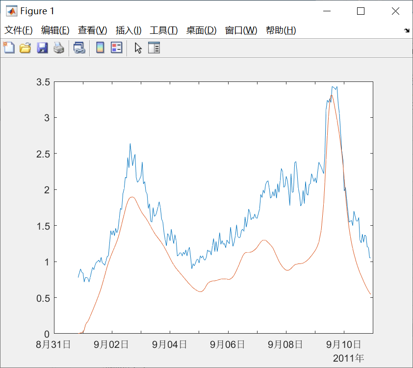
如何画datetime的时序图

如何保存图形（figure）到mat（table, cell）

【小学】MyLifeStyle(3079779149)  17:15:08
请问，matlab中在某个figure上画了图形，关闭figure后，如何再次调出图形？想达到的目的是，像显示变量一样的显示图形~~谢谢~~

【管理员】新疆+源代码+奋斗(535512013)  17:16:00
关闭哪个就在命令框中输入figure几

【小学】MyLifeStyle(3079779149)  17:21:07
关闭后打不开，显示句柄已经删除了，不知道什么意思~~

【管理员】新疆+源代码+奋斗(535512013)  17:23:32
删除和关闭不一样

【管理员】新疆+源代码+奋斗(535512013)  17:27:32
不能重新画吗

【小学】MyLifeStyle(3079779149)  17:29:24
额，是批量画图，一个对象有2个图，总共有200个对象，在分析时才具体看图形~~

【小学】MyLifeStyle(3079779149)  17:30:04
相像保存和调用数据那样，实现图形的保存和调用~

【管理员】新疆+源代码+奋斗(535512013)  17:31:01
只能重新画，把删除命令去掉

【管理员】新疆+源代码+奋斗(535512013)  17:31:13
不然画好了也给你删除了

【小学】MyLifeStyle(3079779149)  17:31:35
好的~~

【管理员】晨雾(914836396)  17:33:39
@MyLifeStyle 你可以直接把fig存下来

【管理员】新疆+源代码+奋斗(535512013)  17:34:56
@MyLifeStyle 大佬来了，他会@晨雾 
【管理员】新疆+源代码+奋斗(535512013)  17:36:39
我就一弟中弟，

【管理员】新疆+源代码+奋斗(535512013)  17:36:49
看见大佬赶紧让路

【小学】MyLifeStyle(3079779149)  17:37:39
看到大佬们都这么谦虚，我又充满了动力

https://ww2.mathworks.cn/help/matlab/ref/savefig.html?s_tid=gn_loc_drop

南海论文的时序图

Step1_Hs_NPJ.m：

tic
clear all
load('Step1_Hs_NPJ')
x = 1958:1:2019;
y = NPJ;

%% The line of best fit
[k1,b1] = Trend_ZuiJiaXianNiHe(x,y);

%% Thei-Sen and MannKendall 
alpha = 0.05;
[k2,b2,k3,b3,k4,b4] = Trend_TheiSenNiHe(x,y,alpha);
[CL,~] = Trend_MannKendallTest(x,y); %置信水平

%% plot
close all
figure('NumberTitle', 'off', 'Name','1','color',[1,1,1])
hold on
plot(x,polyval([k1,b1],x),'r');
plot(x,polyval([k2,b2],x),'k');
plot(x,polyval([k3,b3],x),'--k');
plot(x,polyval([k4,b4],x),'--k');
plot(x,y,'k');
ylabel("mean SWH (m)",'FontName','Times New Roman')

xlim([1957 2020])

% ：：坐标轴设置
while(1)
    x = xlim();
    y = ylim();
    axis([x(1) x(end) y(1) y(end)]); %设置坐标轴axis取值范围
    set(gca,'Tickdir','out'); %设置刻度外翻
    % ：：图形框右边和上边设置
    plot([x(end) x(end)],[y(1) y(end)],...
        'color','k',...
        'linewidth',1);
    plot([x(1) x(end)],[y(end) y(end)],...
        'color','k',...
        'linewidth',1);
    % ：：图形下边和左边
    plot([x(1) x(end)],[y(1) y(1)],...
        'color','k',...
        'linewidth',1);
    plot([x(1) x(1)],[y(1) y(end)],...
        'color','k',...
        'linewidth',1);
    % ：：去掉右上角刻度
    % get(gca)
  
    %
    break
end
%
legend('d','T','T±CL','Location','NorthWest')

toc

南海论文的散点图

SWH_buoy_era5_dat.mat:

链接：https://pan.baidu.com/s/1Oio3VAkl6-KcW8hWQpr51w
提取码：4mib
–来自百度网盘超级会员V5的分享

plot_era5_py301_jieguo.m：

clear all
close all
clc
% data=load('ERA5_PY301_match.dat');
load('SWH_buoy_era5_dat.mat')
a = obs_all;
b = reana_all;
%load('SWH_buoy_era5_dat_2011')
%c = obs_all;
%d = reana_all;
%clear obs_all
%clear reana_all
ndbc_swh = [a];
era5_swh = [b];

[d,de]=DensScat(ndbc_swh,era5_swh); %1
set(gca,'xlim',[0,8],'ylim',[0,8],'fontsize',14,'fontname','Times New Roman')
colormap('Jet')
hc = colorbar;
set(hc,'ticks',[10 40 80 120 160 200 240],'ticklabels',[{'10'};{'40'};{'80'};{'120'};{'160'};{'200'};{'240'};],...
    'LineWidth',1,...
    'fontname','times new roman','FontSize',14,...
    'TickLabelInterpreter','tex',...
    'visible','on');
set(hc.Label,'String','Number of points','fontname','times new roman','FontSize',14);
%hc.Label.String = 'Number of points';
hold on
plot(0:0.01:9,0:0.01:9,'k-','linewidth',2)
xlabel('Buoy SWH (m)','fontsize',14,'fontname','Times New Roman')
ylabel('ERA5 SWH (m)','fontsize',14,'fontname','Times New Roman')

N=length(ndbc_swh);

%[bias,rms,corr]=cal_index(N,ndbc_swh,era5_swh); %2
error = ndbc_swh-era5_swh;
rmse = sqrt(mean(error.*error)) %N
maxBouySWH = max(ndbc_swh)
rmse_max = rmse/maxBouySWH
bias = mean(-1*error)
r = min(min(corrcoef(ndbc_swh, era5_swh)))


hold on
text(1,6.8,['Bias = -0.07 m'],'fontsize',14,'fontname','Times New Roman')
hold on
text(1,7.5,['RMSE = 0.35 m (5.06%)'],'fontsize',14,'fontname','Times New Roman')
hold on
text(1,6.1,['R = 0.95'],'fontsize',14,'fontname','Times New Roman')

DensScat.m：

function [fh,density] = DensScat(x,y, varargin)
% USAGE:
%  fh = DensScat(x, y) makes a density scatter plot using the vectors x & y
%
% INPUTS:
% * x & y are two numeric vectors describing the x-axis & y-axis
% location for each point in the scatter plot
%
% OUTPUTS:
% * fh: figure handle to for the scatter plot
%
% OTHER PARAMETERS passed as parameter-value pairs, defaults in []
% 'MarkerType': Marker type '.od<>^vs+*xph' ['.']
% 'mSize': Integer for Marker size [50 for '.' otherwise 12]
% 'ColorMap': Colormap to be used name eg 'jet' or N*3 matrix [TurboMap]
% 'logDensity': true/false for taking the log10 of the density [true]
% 'AxisSquare': true/false for making axis square [true]
% 'SmoothDensity': true/false for density smoothing [true]
% 'lambda':  Integer for the degree of smoothing [30]
% 'nBin_x': Integer for number of bins along the x-axis [200]
% 'nBin_y': Integer for number of bins along the y-axis [200]
% 'RemovePoints': true/false only plot points that that are unique based
%                 on a 1000*1000 grid [true]
% 'TargetAxes': Axes handle to existing axes that will be used [false]
% 'ColorBar': true/false creates a color bar for the density [true]
% 'MaxDens': double for thresholding density D(D>MaxDens) = MaxDens [inf]
% 'PointsToExclude': Nx2 matrix describing points to be exluded for example
% [0 0] may be useful for RNAseq data [ [] ]
%
% The smoothing is based on the following reference:
% Paul H. C. Eilers and Jelle J. Goeman
% Enhancing scatterplots with smoothed densities
% Bioinformatics, Mar 2004; 20: 623 - 628.
%
%%%%%%%%%%%%%%%%%%%%%%%%%%%%%%%%%%%%%%%%%%%%%%%%%%%%%%%%%%%%%%%%%%%%%%%%%%%
%%% by Anders Berglund, 2020 aebergl@gmail.com                            %
%%%%%%%%%%%%%%%%%%%%%%%%%%%%%%%%%%%%%%%%%%%%%%%%%%%%%%%%%%%%%%%%%%%%%%%%%%%

% Check number of input parameters
if nargin < 2
    error('DensScat requires at least two input vectors');
end

% Check that they are numeric
if ~ismatrix(x) || ~isnumeric(x) || ~ismatrix(y) || ~isnumeric(y)
    error('x & y need to be numeric vectors');
end

% Check that they are all vectors
if min(size(x)) ~= 1 || min(size(x)) ~= 1
    error('x & y must be vectors');
end

% Check that x and Y are of equal length
if (length(x) ~= length(y))
    error('x & y must all have equal length');
end

% Make sure that x & y are all column vectors and not row vectors
if size(x,1) == 1
    x = x';
end
if size(y,1) == 1
    y = y';
end

%Parse input and set default values
p = parseArguments(varargin{:});

fh = 0;

% Remove Missing values
indx = isnan(x) | isnan(y);
x(indx)= [];
y(indx)= [];

if ~isempty(p.PointsToExclude)
    for i=1:size(p.PointsToExclude,1)
        indx = (x == p.PointsToExclude(i,1)) & (y == p.PointsToExclude(i,2));
        x(indx)= [];
        y(indx)= [];
    end
end

% get ranges
min_x = min(x);
max_x = max(x);
min_y = min(y);
max_y = max(y);


% Define edges
edges_x = linspace(min_x, max_x, p.nBin_x+1);
edges_x([ 1 end]) = [-Inf +Inf];
edges_y = linspace(min_y, max_y, p.nBin_y+1);
edges_y([ 1 end]) = [-Inf +Inf];

% Get number of counts
[~,~,~,bin(:,2),bin(:,1)] = histcounts2(x,y,edges_x,edges_y);

H = accumarray(bin,1,[p.nBin_y p.nBin_x]);

% Smoothing
if p.SmoothDensity
    H = smooth1D(H,p.nBin_y/p.lambda);
    H = smooth1D(H',p.nBin_x/p.lambda)';
end

% Get density for each point
ind = sub2ind(size(H),bin(:,1),bin(:,2));
density = H(ind);
if p.logDensity
    density = log10(density+1);
end

if p.MaxDens
    density(density > p.MaxDens) = p.MaxDens;
end

% make sure that high density points are plotted last
[density,sort_indx] = sort(density,'Ascend');
x = x(sort_indx);
y = y(sort_indx);

if p.RemovePoints
    x = round(x,3,'Significant');
    y = round(y,3,'Significant');
    [~,indx,~] = unique([x, y],'rows','stable');
    x = x(indx);
    y = y(indx);
    density = density(indx);
end

if isgraphics(p.TargetAxes,'axes')
    ah = p.TargetAxes;
else
    % Create figure handle
    fh = figure('Name','Density Scatter Plot','Color','w','Tag','Density Scatter Plot','GraphicsSmoothing','off');
    % Create figure handle
    ah = axes(fh,'NextPlot','add','tag','Scatter Plot','Box','on','FontSize',16,'Linewidth',1);
end

if ismatrix(p.ColorMap) && isnumeric(p.ColorMap)
    cMap = p.ColorMap;
elseif strcmpi(p.ColorMap,'TurboMap')
    cMap = TurboMap;
else
    cMap=colormap(p.ColorMap);
end

colormap(cMap);

scatter(ah,x,y,p.mSize,density,p.MarkerType);

if p.AxisSquare
    axis square
end

if p.ColorBar
    hc = colorbar(ah);
    hc.Label.String = 'Density';
end


end

function p = parseArguments(varargin)
p = inputParser;

expectedMarkerType = {'.od<>^vs+*xph'};

addParameter(p,'MarkerType', '.', @(x) length(x)==1 && ~isempty((strfind(expectedMarkerType,x))));
addParameter(p,'mSize', 50, @(x) isnumeric(x) && isscalar(x) && x > 0);
addParameter(p,'ColorMap', 'TurboMap');
addParameter(p,'logDensity', false, @islogical);
addParameter(p,'AxisSquare', false, @islogical);
addParameter(p,'SmoothDensity', true, @islogical);
addParameter(p,'lambda', 30, @(x) isnumeric(x) && isscalar(x) && x > 0);
addParameter(p,'nBin_x', 100, @(x) isnumeric(x) && isscalar(x) && x > 0);
addParameter(p,'nBin_y', 100, @(x) isnumeric(x) && isscalar(x) && x > 0);
addParameter(p,'RemovePoints', true, @islogical);
addParameter(p,'TargetAxes', false, @(x) isgraphics(x,'axes'));
addParameter(p,'ColorBar', false, @islogical);
addParameter(p,'MaxDens', inf, @(x) isnumeric(x) && isscalar(x) && x > 0);
addParameter(p,'PointsToExclude', [], @(x) isnumeric(x))


parse(p,varargin{:});
p = p.Results;

if ~p.MarkerType == '.'
    p.mSize = 12;
end
end

function Z = smooth1D(X,lambda)
% The smoothing is based on the following reference:
% Paul H. C. Eilers and Jelle J. Goeman
% Enhancing scatterplots with smoothed densities
% Bioinformatics, Mar 2004; 20: 623 - 628.

[n] = size(X,1);
E = eye(n);
D1 = diff(E,1);
D2 = diff(D1,1);
P = lambda.^2 .* D2'*D2 + 2.*lambda .* D1'*D1;
Z = (E + P) \ X;

end

function CMap = TurboMap
% https://ai.googleblog.com/2019/08/turbo-improved-rainbow-colormap-for.html

CMap = [
    0.18995      0.07176      0.23217
    0.19483      0.08339      0.26149
    0.19956      0.09498      0.29024
    0.20415      0.10652      0.31844
    0.2086      0.11802      0.34607
    0.21291      0.12947      0.37314
    0.21708      0.14087      0.39964
    0.22111      0.15223      0.42558
    0.225      0.16354      0.45096
    0.22875      0.17481      0.47578
    0.23236      0.18603      0.50004
    0.23582       0.1972      0.52373
    0.23915      0.20833      0.54686
    0.24234      0.21941      0.56942
    0.24539      0.23044      0.59142
    0.2483      0.24143      0.61286
    0.25107      0.25237      0.63374
    0.25369      0.26327      0.65406
    0.25618      0.27412      0.67381
    0.25853      0.28492        0.693
    0.26074      0.29568      0.71162
    0.2628      0.30639      0.72968
    0.26473      0.31706      0.74718
    0.26652      0.32768      0.76412
    0.26816      0.33825       0.7805
    0.26967      0.34878      0.79631
    0.27103      0.35926      0.81156
    0.27226       0.3697      0.82624
    0.27334      0.38008      0.84037
    0.27429      0.39043      0.85393
    0.27509      0.40072      0.86692
    0.27576      0.41097      0.87936
    0.27628      0.42118      0.89123
    0.27667      0.43134      0.90254
    0.27691      0.44145      0.91328
    0.27701      0.45152      0.92347
    0.27698      0.46153      0.93309
    0.2768      0.47151      0.94214
    0.27648      0.48144      0.95064
    0.27603      0.49132      0.95857
    0.27543      0.50115      0.96594
    0.27469      0.51094      0.97275
    0.27381      0.52069      0.97899
    0.27273       0.5304      0.98461
    0.27106      0.54015       0.9893
    0.26878      0.54995      0.99303
    0.26592      0.55979      0.99583
    0.26252      0.56967      0.99773
    0.25862      0.57958      0.99876
    0.25425       0.5895      0.99896
    0.24946      0.59943      0.99835
    0.24427      0.60937      0.99697
    0.23874      0.61931      0.99485
    0.23288      0.62923      0.99202
    0.22676      0.63913      0.98851
    0.22039      0.64901      0.98436
    0.21382      0.65886      0.97959
    0.20708      0.66866      0.97423
    0.20021      0.67842      0.96833
    0.19326      0.68812       0.9619
    0.18625      0.69775      0.95498
    0.17923      0.70732      0.94761
    0.17223       0.7168      0.93981
    0.16529       0.7262      0.93161
    0.15844      0.73551      0.92305
    0.15173      0.74472      0.91416
    0.14519      0.75381      0.90496
    0.13886      0.76279       0.8955
    0.13278      0.77165       0.8858
    0.12698      0.78037       0.8759
    0.12151      0.78896      0.86581
    0.11639       0.7974      0.85559
    0.11167      0.80569      0.84525
    0.10738      0.81381      0.83484
    0.10357      0.82177      0.82437
    0.10026      0.82955      0.81389
    0.0975      0.83714      0.80342
    0.09532      0.84455      0.79299
    0.09377      0.85175      0.78264
    0.09287      0.85875       0.7724
    0.09267      0.86554       0.7623
    0.0932      0.87211      0.75237
    0.09451      0.87844      0.74265
    0.09662      0.88454      0.73316
    0.09958       0.8904      0.72393
    0.10342        0.896        0.715
    0.10815      0.90142      0.70599
    0.11374      0.90673      0.69651
    0.12014      0.91193       0.6866
    0.12733      0.91701      0.67627
    0.13526      0.92197      0.66556
    0.14391       0.9268      0.65448
    0.15323      0.93151      0.64308
    0.16319      0.93609      0.63137
    0.17377      0.94053      0.61938
    0.18491      0.94484      0.60713
    0.19659      0.94901      0.59466
    0.20877      0.95304      0.58199
    0.22142      0.95692      0.56914
    0.23449      0.96065      0.55614
    0.24797      0.96423      0.54303
    0.2618      0.96765      0.52981
    0.27597      0.97092      0.51653
    0.29042      0.97403      0.50321
    0.30513      0.97697      0.48987
    0.32006      0.97974      0.47654
    0.33517      0.98234      0.46325
    0.35043      0.98477      0.45002
    0.36581      0.98702      0.43688
    0.38127      0.98909      0.42386
    0.39678      0.99098      0.41098
    0.41229      0.99268      0.39826
    0.42778      0.99419      0.38575
    0.44321      0.99551      0.37345
    0.45854      0.99663       0.3614
    0.47375      0.99755      0.34963
    0.48879      0.99828      0.33816
    0.50362      0.99879      0.32701
    0.51822       0.9991      0.31622
    0.53255      0.99919      0.30581
    0.54658      0.99907      0.29581
    0.56026      0.99873      0.28623
    0.57357      0.99817      0.27712
    0.58646      0.99739      0.26849
    0.59891      0.99638      0.26038
    0.61088      0.99514       0.2528
    0.62233      0.99366      0.24579
    0.63323      0.99195      0.23937
    0.64362      0.98999      0.23356
    0.65394      0.98775      0.22835
    0.66428      0.98524       0.2237
    0.67462      0.98246       0.2196
    0.68494      0.97941      0.21602
    0.69525       0.9761      0.21294
    0.70553      0.97255      0.21032
    0.71577      0.96875      0.20815
    0.72596       0.9647       0.2064
    0.7361      0.96043      0.20504
    0.74617      0.95593      0.20406
    0.75617      0.95121      0.20343
    0.76608      0.94627      0.20311
    0.77591      0.94113       0.2031
    0.78563      0.93579      0.20336
    0.79524      0.93025      0.20386
    0.80473      0.92452      0.20459
    0.8141      0.91861      0.20552
    0.82333      0.91253      0.20663
    0.83241      0.90627      0.20788
    0.84133      0.89986      0.20926
    0.8501      0.89328      0.21074
    0.85868      0.88655       0.2123
    0.86709      0.87968      0.21391
    0.8753      0.87267      0.21555
    0.88331      0.86553      0.21719
    0.89112      0.85826       0.2188
    0.8987      0.85087      0.22038
    0.90605      0.84337      0.22188
    0.91317      0.83576      0.22328
    0.92004      0.82806      0.22456
    0.92666      0.82025       0.2257
    0.93301      0.81236      0.22667
    0.93909      0.80439      0.22744
    0.94489      0.79634        0.228
    0.95039      0.78823      0.22831
    0.9556      0.78005      0.22836
    0.96049      0.77181      0.22811
    0.96507      0.76352      0.22754
    0.96931      0.75519      0.22663
    0.97323      0.74682      0.22536
    0.97679      0.73842      0.22369
    0.98         0.73      0.22161
    0.98289       0.7214      0.21918
    0.98549       0.7125       0.2165
    0.98781       0.7033      0.21358
    0.98986      0.69382      0.21043
    0.99163      0.68408      0.20706
    0.99314      0.67408      0.20348
    0.99438      0.66386      0.19971
    0.99535      0.65341      0.19577
    0.99607      0.64277      0.19165
    0.99654      0.63193      0.18738
    0.99675      0.62093      0.18297
    0.99672      0.60977      0.17842
    0.99644      0.59846      0.17376
    0.99593      0.58703      0.16899
    0.99517      0.57549      0.16412
    0.99419      0.56386      0.15918
    0.99297      0.55214      0.15417
    0.99153      0.54036       0.1491
    0.98987      0.52854      0.14398
    0.98799      0.51667      0.13883
    0.9859      0.50479      0.13367
    0.9836      0.49291      0.12849
    0.98108      0.48104      0.12332
    0.97837       0.4692      0.11817
    0.97545       0.4574      0.11305
    0.97234      0.44565      0.10797
    0.96904      0.43399      0.10294
    0.96555      0.42241      0.09798
    0.96187      0.41093       0.0931
    0.95801      0.39958      0.08831
    0.95398      0.38836      0.08362
    0.94977      0.37729      0.07905
    0.94538      0.36638      0.07461
    0.94084      0.35566      0.07031
    0.93612      0.34513      0.06616
    0.93125      0.33482      0.06218
    0.92623      0.32473      0.05837
    0.92105      0.31489      0.05475
    0.91572       0.3053      0.05134
    0.91024      0.29599      0.04814
    0.90463      0.28696      0.04516
    0.89888      0.27824      0.04243
    0.89298      0.26981      0.03993
    0.88691      0.26152      0.03753
    0.88066      0.25334      0.03521
    0.87422      0.24526      0.03297
    0.8676       0.2373      0.03082
    0.86079      0.22945      0.02875
    0.8538       0.2217      0.02677
    0.84662      0.21407      0.02487
    0.83926      0.20654      0.02305
    0.83172      0.19912      0.02131
    0.82399      0.19182      0.01966
    0.81608      0.18462      0.01809
    0.80799      0.17753       0.0166
    0.79971      0.17055       0.0152
    0.79125      0.16368      0.01387
    0.7826      0.15693      0.01264
    0.77377      0.15028      0.01148
    0.76476      0.14374      0.01041
    0.75556      0.13731      0.00942
    0.74617      0.13098      0.00851
    0.73661      0.12477      0.00769
    0.72686      0.11867      0.00695
    0.71692      0.11268      0.00629
    0.7068       0.1068      0.00571
    0.6965      0.10102      0.00522
    0.68602      0.09536      0.00481
    0.67535       0.0898      0.00449
    0.66449      0.08436      0.00424
    0.65345      0.07902      0.00408
    0.64223       0.0738      0.00401
    0.63082      0.06868      0.00401
    0.61923      0.06367       0.0041
    0.60746      0.05878      0.00427
    0.5955      0.05399      0.00453
    0.58336      0.04931      0.00486
    0.57103      0.04474      0.00529
    0.55852      0.04028      0.00579
    0.54583      0.03593      0.00638
    0.53295      0.03169      0.00705
    0.51989      0.02756       0.0078
    0.50664      0.02354      0.00863
    0.49321      0.01963      0.00955
    0.4796      0.01583      0.01055
    ];

end

运行结果：

second, ndbc_station_download_NC_analyse

% author:
%    liu jin can, UPC
%
% revison history
%    2022-02-18 first verison.
%    2022-02-18 second, ndbc_station_download_NC_analyse

clc, clear all
%load ndbc_station_download_NC.mat
load ndbc_station_download_NC_analyse; ndbc_station_download_NC = ndbc_station_download_NC_analyse;
disp('已加载ndbc_station_download_NC.mat！'); pause(1);


%% 时间-WVHT数据，一个小时一个数据
%-----------------------------
%参数
path_fig = '.\fig\'; %%https://ww2.mathworks.cn/help/matlab/ref/savefig.html?s_tid=gn_loc_drop
%-----------------------------

for i=[29]%1:1:size(ndbc_station_download_NC,1)
    disp(strcat(ndbc_station_download_NC.station_ID{i},'时间-WVHT数据分析，一个小时一个数据：'));
    %% 去除ndbc数据table无效数据所在行
    ndbc_table = ndbc_station_download_NC.station_historyData_SM{i,1}; %table
    ndbc_WVHT1 = cell2mat(ndbc_table.WVHT(:)); %double
    ndbc_time1 = ndbc_table.YY_MM_DD_hh_mm; % datetime
    tf1 = find( ndbc_WVHT1>=0 & ndbc_WVHT1<99 );
  
    ndbc_time2 = ndbc_time1(tf1);
    ndbc_WVHT2 = ndbc_WVHT1(tf1);
    disp(strcat('      已去除ndbc数据table无效数据所在行；'));
    %% ndbc数据，一个小时一个数据
    % 超过30分钟，进一个小时
    tf2 = find( ndbc_time2.Minute>30 & ndbc_time2.Minute<60 ); % case1, 秒数都是0，因为ndbc不包含秒数信息；
    temp = ndbc_time2(tf2); temp.Minute = 0; temp.Hour = temp.Hour+1;
    ndbc_time2(tf2) = temp;
    % 少于30分钟，小时不变
    tf3 = find( ndbc_time2.Minute>0 & ndbc_time2.Minute<30 ); % case2；
    temp = ndbc_time2(tf3); temp.Minute = 0;
    ndbc_time2(tf3) = temp;
    % 年、月、日、时相等的datetime处理：
    count = tabulate(ndbc_time2); % 统计数列中每个元素出现的次数
    tf4 = find(cell2mat(count(:,2))>1); % 元素次数超过1次
    for j=1:1:size(tf4,1) %元素次数超过1次的元素进行平均化处理
        temp = datetime(count{tf4(j),1});
        tf5 = find(ndbc_time2==temp);
        ndbc_WVHT2(tf5(1)) = mean(ndbc_WVHT2(tf5)); %平均化处理
        ndbc_WVHT2(tf5(2:end)) = 99; %无效数据
        % ndbc_WVHT2(tf5)
    end
    tf6 = find( ndbc_WVHT2>=0 & ndbc_WVHT2<99 );
    ndbc_time3 = ndbc_time2(tf6); % unique(ndbc_time3); %通过维数不变，发现每一个元素都是唯一的;
    ndbc_WVHT3 = ndbc_WVHT2(tf6);
    disp(strcat('      已实现ndbc数据，一个小时一个数据，（通过了unique(ndbc_time3)的检验）；'));
    %% nc 数据，一个小时一个数据；
    disp(strcat('      已确定nc数据，一个小时一个数据；'));
    %% ndbc 和 nc 小时数据匹配；
    % 组合ndbc和nc的数据
    temp = ndbc_station_download_NC.nc_time_WVHT{i,1};
    ndbc_nc_time = [ndbc_time3;temp{:,1}]; %ndbc 和 nc的datetime数据组合
    ndbc_nc_WVHT = [ndbc_WVHT3;temp{:,2}]; %ndbc 和 nc的WVHT数据组合
    % 匹配
    ndbc_nc_match_WVHT = table;
    count = tabulate(ndbc_nc_time); %匹配的时间元素，会出现2次，而且不可能超过两次；
    tf7 = find(cell2mat(count(:,2))>1); % 元素次数超过1次
    temp1 = []; %存储时间
    temp2 = []; %存储ndbc数据
    temp3 = []; %存储nc数据
    for j=1:1:size(tf7,1)
        temp = datetime(count{tf7(j),1});
        tf8 = find(ndbc_nc_time==temp);
        temp1 = [temp1;temp];
        temp2 = [temp2;ndbc_nc_WVHT(tf8(1))];
        temp3 = [temp3;ndbc_nc_WVHT(tf8(2))];
    end
    ndbc_nc_match_WVHT.time = temp1;
    ndbc_nc_match_WVHT.ndbc = temp2;
    ndbc_nc_match_WVHT.nc = temp3;
    disp(strcat('      已对 ndbc 和 nc 小时数据匹配；'));
    %% 匹配数据分析
    if size(tf7,1)<3
        disp(strcat('      发现',ndbc_station_download_NC.station_ID{i},'匹配的数据不足3个'));pause(1);
        ndbc_station_download_NC.ndbc_nc_match_WVHT{i,1} = strcat('      发现',ndbc_station_download_NC.station_ID{i},'匹配的数据不足3个');
    else
        % 时序图
        f = figure(1);
        plot(ndbc_nc_match_WVHT.time,ndbc_nc_match_WVHT.ndbc);
        hold on; plot(ndbc_nc_match_WVHT.time,ndbc_nc_match_WVHT.nc);
        %close(f1)
        savefig(f,strcat(path_fig,ndbc_station_download_NC.station_ID{i},'一小时时间-WVHT数据-时序图','.fig')); %https://ww2.mathworks.cn/help/matlab/ref/savefig.html?s_tid=gn_loc_drop
        ndbc_nc_match_WVHT.TimeSeriesChart{1,1} = strcat('openfig("',path_fig,ndbc_station_download_NC.station_ID{i},'一小时时间-WVHT数据-时序图','.fig")');
        close(f)
        %openfig('1.fig');
        disp(strcat('      已简单画出时序图，并保存;'));
      
        % rmse, bias, R, SI, PE
        error = ndbc_nc_match_WVHT.ndbc-ndbc_nc_match_WVHT.nc;
        rmse = sqrt(mean(error.*error));
        bias = mean(-1*error);
        r = min(min(corrcoef(ndbc_nc_match_WVHT.ndbc, ndbc_nc_match_WVHT.nc)));
        PE = sqrt(mean((error./ndbc_nc_match_WVHT.ndbc).^2))*100;
        SI = rmse/mean(ndbc_nc_match_WVHT.ndbc);
      
        ndbc_nc_match_WVHT.rmse{1,1} = rmse;
        ndbc_nc_match_WVHT.bias{1,1} = bias;
        ndbc_nc_match_WVHT.r{1,1} = r;
        ndbc_nc_match_WVHT.PE{1,1} = PE;
        ndbc_nc_match_WVHT.SI{1,1} = SI;
        disp(strcat('      已计算RMSE, BIAS, R, SI, PE，并保存;'));
      
      
      
        % 散点图
        [f,de] = DensScat(ndbc_nc_match_WVHT.ndbc,ndbc_nc_match_WVHT.nc);
        colormap('Jet')
        hc = colorbar;
        savefig(f,strcat(path_fig,ndbc_station_download_NC.station_ID{i},'一小时时间-WVHT数据-散点图','.fig'));
        ndbc_nc_match_WVHT.ScatterChart{1,1} = strcat('openfig("',path_fig,ndbc_station_download_NC.station_ID{i},'一小时时间-WVHT数据-散点图','.fig")');
        close(f)
        disp(strcat('      已简单画出散点图，并保存;'));
      
        % 保存到总的table
        ndbc_station_download_NC.ndbc_nc_match_WVHT{i,1} = ndbc_nc_match_WVHT;
    end
  
  
end

%%
%ndbc_station_download_NC_analyse = ndbc_station_download_NC;
%save ndbc_station_download_NC_analyse ndbc_station_download_NC_analyse

third, function, path_save, 图床思想

function [ndbc_station_download_NC] = ndbc_station_download_NC_analyse(ndbc_station_download_NC,station_tf_download,path_save)
% author:
%    liu jin can, UPC
%
% revison history
%    2022-02-18 first verison.
%    2022-02-18 second, ndbc_station_download_NC_analyse
%    2022-02-19 third, function, path_save.
%    2022-02-19        图床思想

%clc, clear all
%load ndbc_station_download_NC.mat
%load ndbc_station_download_NC_analyse; ndbc_station_download_NC = ndbc_station_download_NC_analyse;
%disp('已加载ndbc_station_download_NC.mat！'); pause(1);

%%
disp('-----------------------ndbc_station_download_NC_analyse')
cd(path_save)


%% 时间-WVHT数据，一个小时一个数据
%-----------------------------
%参数
path_fig = '.\fig\'; %%https://ww2.mathworks.cn/help/matlab/ref/savefig.html?s_tid=gn_loc_drop
%-----------------------------

for i=station_tf_download%1:1:size(ndbc_station_download_NC,1)
    disp(strcat(ndbc_station_download_NC.station_ID{i},'时间-WVHT数据分析，一个小时一个数据：'));
    %% 去除ndbc数据table无效数据所在行
    temp = strcat(path_save,'station_historyData_SM\',num2str(i),'.mat');
    load(temp); % temp 中仅有 buoy_table_All 变量；
    %ndbc_table = ndbc_station_download_NC.station_historyData_SM{i,1}; %table
    ndbc_table = buoy_table_All;
    ndbc_WVHT1 = cell2mat(ndbc_table.WVHT(:)); %double
    ndbc_time1 = ndbc_table.YY_MM_DD_hh_mm; % datetime
    tf1 = find( ndbc_WVHT1>=0 & ndbc_WVHT1<99 );
  
    ndbc_time2 = ndbc_time1(tf1);
    ndbc_WVHT2 = ndbc_WVHT1(tf1);
    disp(strcat('      已去除ndbc数据table无效数据所在行；'));
    %% ndbc数据，一个小时一个数据
    % 超过30分钟，进一个小时
    tf2 = find( ndbc_time2.Minute>30 & ndbc_time2.Minute<60 ); % case1, 秒数都是0，因为ndbc不包含秒数信息；
    temp = ndbc_time2(tf2); temp.Minute = 0; temp.Hour = temp.Hour+1;
    ndbc_time2(tf2) = temp;
    % 少于30分钟，小时不变
    tf3 = find( ndbc_time2.Minute>0 & ndbc_time2.Minute<30 ); % case2；
    temp = ndbc_time2(tf3); temp.Minute = 0;
    ndbc_time2(tf3) = temp;
    % 年、月、日、时相等的datetime处理：
    count = tabulate(ndbc_time2); % 统计数列中每个元素出现的次数
    tf4 = find(cell2mat(count(:,2))>1); % 元素次数超过1次
    for j=1:1:size(tf4,1) %元素次数超过1次的元素进行平均化处理
        temp = datetime(count{tf4(j),1});
        tf5 = find(ndbc_time2==temp);
        ndbc_WVHT2(tf5(1)) = mean(ndbc_WVHT2(tf5)); %平均化处理
        ndbc_WVHT2(tf5(2:end)) = 99; %无效数据
        % ndbc_WVHT2(tf5)
    end
    tf6 = find( ndbc_WVHT2>=0 & ndbc_WVHT2<99 );
    ndbc_time3 = ndbc_time2(tf6); % unique(ndbc_time3); %通过维数不变，发现每一个元素都是唯一的;
    ndbc_WVHT3 = ndbc_WVHT2(tf6);
    disp(strcat('      已实现ndbc数据，一个小时一个数据，（通过了unique(ndbc_time3)的检验）；'));
    %% nc 数据，一个小时一个数据；
    disp(strcat('      已确定nc数据，一个小时一个数据；'));
    %% ndbc 和 nc 小时数据匹配；
    % 组合ndbc和nc的数据
    temp = ndbc_station_download_NC.nc_time_WVHT{i,1};
    ndbc_nc_time = [ndbc_time3;temp{:,1}]; %ndbc 和 nc的datetime数据组合
    ndbc_nc_WVHT = [ndbc_WVHT3;temp{:,2}]; %ndbc 和 nc的WVHT数据组合
    % 匹配
    ndbc_nc_match_WVHT = table;
    count = tabulate(ndbc_nc_time); %匹配的时间元素，会出现2次，而且不可能超过两次；
    tf7 = find(cell2mat(count(:,2))>1); % 元素次数超过1次
    temp1 = []; %存储时间
    temp2 = []; %存储ndbc数据
    temp3 = []; %存储nc数据
    for j=1:1:size(tf7,1)
        temp = datetime(count{tf7(j),1});
        tf8 = find(ndbc_nc_time==temp);
        temp1 = [temp1;temp];
        temp2 = [temp2;ndbc_nc_WVHT(tf8(1))];
        temp3 = [temp3;ndbc_nc_WVHT(tf8(2))];
    end
    ndbc_nc_match_WVHT.time = temp1;
    ndbc_nc_match_WVHT.ndbc = temp2;
    ndbc_nc_match_WVHT.nc = temp3;
    disp(strcat('      已对 ndbc 和 nc 小时数据匹配；'));
    %% 匹配数据分析
    if size(tf7,1)<3
        disp(strcat('      发现',ndbc_station_download_NC.station_ID{i},'匹配的数据不足3个'));pause(1);
        ndbc_station_download_NC.ndbc_nc_match_WVHT{i,1} = strcat('      发现',ndbc_station_download_NC.station_ID{i},'匹配的数据不足3个');
    else
        % 时序图
        f = figure(1);
        plot(ndbc_nc_match_WVHT.time,ndbc_nc_match_WVHT.ndbc);
        hold on; plot(ndbc_nc_match_WVHT.time,ndbc_nc_match_WVHT.nc);
        %close(f1)
        savefig(f,strcat(path_fig,ndbc_station_download_NC.station_ID{i},'一小时时间-WVHT数据-时序图','.fig')); %https://ww2.mathworks.cn/help/matlab/ref/savefig.html?s_tid=gn_loc_drop
        ndbc_nc_match_WVHT.TimeSeriesChart{1,1} = strcat('openfig("',path_fig,ndbc_station_download_NC.station_ID{i},'一小时时间-WVHT数据-时序图','.fig")');
        close(f)
        %openfig('1.fig');
        disp(strcat('      已简单画出时序图，并保存;'));
      
        % rmse, bias, R, SI, PE
        error = ndbc_nc_match_WVHT.ndbc-ndbc_nc_match_WVHT.nc;
        rmse = sqrt(mean(error.*error));
        bias = mean(-1*error);
        r = min(min(corrcoef(ndbc_nc_match_WVHT.ndbc, ndbc_nc_match_WVHT.nc)));
        PE = sqrt(mean((error./ndbc_nc_match_WVHT.ndbc).^2))*100;
        SI = rmse/mean(ndbc_nc_match_WVHT.ndbc);
      
        ndbc_nc_match_WVHT.rmse{1,1} = rmse;
        ndbc_nc_match_WVHT.bias{1,1} = bias;
        ndbc_nc_match_WVHT.r{1,1} = r;
        ndbc_nc_match_WVHT.PE{1,1} = PE;
        ndbc_nc_match_WVHT.SI{1,1} = SI;
        disp(strcat('      已计算RMSE, BIAS, R, SI, PE，并保存;'));
      
      
      
        % 散点图
        [f,de] = DensScat(ndbc_nc_match_WVHT.ndbc,ndbc_nc_match_WVHT.nc);
        colormap('Jet')
        hc = colorbar;
        savefig(f,strcat(path_fig,ndbc_station_download_NC.station_ID{i},'一小时时间-WVHT数据-散点图','.fig'));
        ndbc_nc_match_WVHT.ScatterChart{1,1} = strcat('openfig("',path_fig,ndbc_station_download_NC.station_ID{i},'一小时时间-WVHT数据-散点图','.fig")');
        close(f)
        disp(strcat('      已简单画出散点图，并保存;'));
      
        % 保存到总的table
        ndbc_station_download_NC.ndbc_nc_match_WVHT{i,1} = ndbc_nc_match_WVHT;
    end
  
  
end

%%
%ndbc_station_download_NC_analyse = ndbc_station_download_NC;
%save ndbc_station_download_NC_analyse ndbc_station_download_NC_analyse

end

对更多的浮标进行整套分析

加载 ndbc_station_download_NC_analyse.mat，可以看到还有很多浮标没有进行整套分析，下面添加的内容都是在 ndbc_station_download_NC_analyse变量基础上实现的。

添加之前画的浮标plot

ndbc_station_info_needed_plot.m：加载ndbc_station_download_NC_analyse.mat，保存fig，在table中添加打开fig的代码字符串，保存ndbc_station_download_NC_analyse；

对一个浮标添加整套分析

ndbc网上查找，发现 MDRM1浮标包含了nc文件的时间段，故用此浮标；（但全是无效的有效波高~~┭┮﹏┭┮）

整套分析如下：

首先是创建一个ndbc_station_download_NC_analyse.mat的副本，以防意外发生时数据缺失；
下载浮标数据；

ndbc_station_download.m：退出clash，重启matlab，加载ndbc_station_download_NC_analyse.mat，更改浮标对应的i索引，运行后保存ndbc_station_download_NC_analyse.mat；
此浮标对应的nc数据；

ndbc_station_download_NC.m：加载ndbc_station_download_NC_analyse.mat，更改浮标对应的i索引，运行后保存ndbc_station_download_NC_analyse.mat；
浮标数据和nc数据匹配+匹配后分析；

ndbc_station_download_NC_analyse.m：加载ndbc_station_download_NC_analyse.mat，更改浮标对应的i索引，运行后保存ndbc_station_download_NC_analyse.mat；

换一个有效浮标 44013，索引9，进行上面的操作；

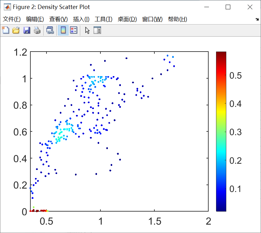
将其余的浮标都进行以上操作，**索引…**；

所以，往后记住，一切的核心数据都在ndbc_station_download_NC_analyse.mat，千万要记住，对其进行操作时，需要备份！！！

NDBC包

NDBC包以文件夹形式存在，文件夹命名为 ndbc；

链接：https://pan.baidu.com/s/1zWesXbLyUi9_l0Udj9EFYA
提取码：vupa
–来自百度网盘超级会员V5的分享

2022-02-19

m_map文件夹

用于进行地图的绘制，需要将此文件夹添加到matlab环境中；

source文件夹

将需要用到的函数放进 source文件夹，将文件夹添加到matlab环境中；

函数要求：

执行程序时，除了ndbc_station_info_needed_plot函数，其它函数不需要进去专门修改参数，参数的修改在work.m文件中实现；
可以实现 work.m既可以在ndbc文件夹下运行，又可以在work文件夹下运行；（解决方法：参数传递添加path_save）

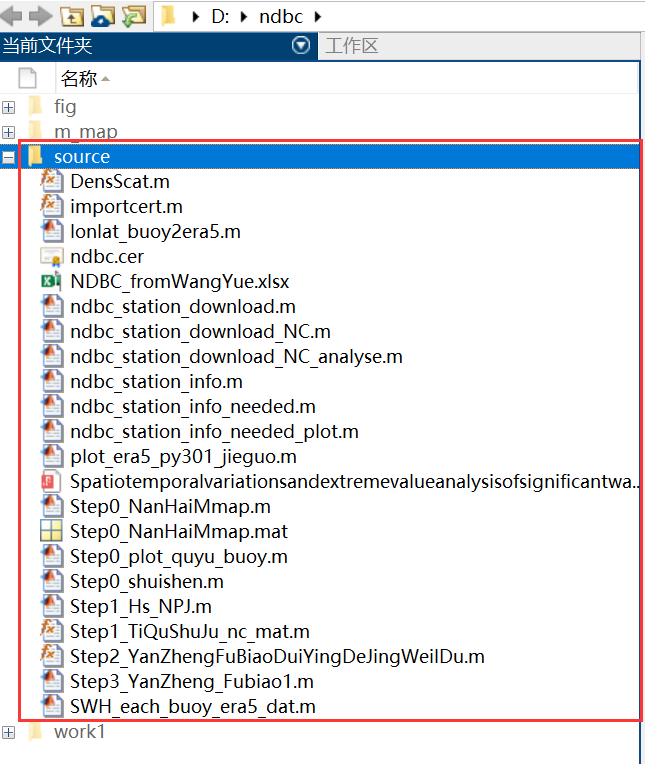
2022-03-03 gantt_year.py （未实现）

在 source 文件夹新添的 gantt_year.py 是为了画出 work_table.mat 中已有浮标关于年份的甘特图。

关于浮标的某一参数有效数据的甘特图，需要打开对应浮标详细的数据，这可能需要时间较久，后面在用另一个函数画这个图吧。

如何使用Python Pandas绘制堆叠事件持续时间（甘特图）？ https://www.cnpython.com/qa/51089

使用Bokeh（一个python库）来制作甘特图，它非常漂亮。这是我从twiiter复制的代码。

No module named ‘bokeh.charts’

What to use instead of bokeh.charts https://stackoverflow.com/questions/48170086/what-to-use-instead-of-bokeh-charts

bokeh库官方-处理分类数据部分：https://docs.bokeh.org/en/latest/docs/user_guide/categorical.html

宝藏库呀~~

时间进度堆叠图；

加载 work_table.mat ，

++++++++++++++++++++++++++++++++

供参考的时间stack图

from bokeh.plotting import figure, show, output_notebook, output_file
from bokeh.models import ColumnDataSource, Range1d
from bokeh.models.tools import HoverTool
from datetime import datetime
#from bokeh.charts import Bar
#output_notebook()
output_file('GanntChart.html') #use this to create a standalone html file to send to others
import pandas as ps

DF=ps.DataFrame(columns=['Item','Start','End','Color'])
Items=[
    ['Contract Review & Award','2015-7-22','2015-8-7','red'],
    ['Submit SOW','2015-8-10','2015-8-14','gray'],
    ['Initial Field Study','2015-8-17','2015-8-21','gray'],
    ['Topographic Procesing','2015-9-1','2016-6-1','gray'],
    ['Init. Hydrodynamic Modeling','2016-1-2','2016-3-15','gray'],
    ['Prepare Suitability Curves','2016-2-1','2016-3-1','gray'],
    ['Improvement Conceptual Designs','2016-5-1','2016-6-1','gray'],
    ['Retrieve Water Level Data','2016-8-15','2016-9-15','gray'],
    ['Finalize Hydrodynamic Models','2016-9-15','2016-10-15','gray'],
    ['Determine Passability','2016-9-15','2016-10-1','gray'],
    ['Finalize Improvement Concepts','2016-10-1','2016-10-31','gray'],
    ['Stakeholder Meeting','2016-10-20','2016-10-21','blue'],
    ['Completion of Project','2016-11-1','2016-11-30','red']
    ] #first items on bottom

for i,Dat in enumerate(Items[::-1]):
    DF.loc[i]=Dat

#convert strings to datetime fields:
DF['Start_dt']=ps.to_datetime(DF.Start)
DF['End_dt']=ps.to_datetime(DF.End)


G=figure(title='Project Schedule',x_axis_type='datetime',width=800,height=400,y_range=DF.Item.tolist(),
        x_range=Range1d(DF.Start_dt.min(),DF.End_dt.max()), tools='save')

hover=HoverTool(tooltips="Task: @Item<br>\
Start: @Start<br>\
End: @End")
G.add_tools(hover)

DF['ID']=DF.index+0.8
DF['ID1']=DF.index+1.2
CDS=ColumnDataSource(DF)
G.quad(left='Start_dt', right='End_dt', bottom='ID', top='ID1',source=CDS,color="Color")
#G.rect(,"Item",source=CDS)
show(G)

bokeh库官方-处理分类数据部分

https://docs.bokeh.org/en/latest/docs/user_guide/categorical.html

使用NDBC包方法：work 文件夹

一个work文件夹对应一个工作空间；

下面是如何使用NDBC包的内容，用的是本次寒假的例子：

至少 matlab 2020a 版本；
将m_map和source文件夹添加到matlab环境；

在ndbc文件夹下新建 work_eastUSA文件夹，再在 work_eastUSA文件夹下新建 work_eastUSA.m，导入所需要的 nc文件；

work_eastUSA.m：

% author:
%    liu jin can, UPC
%
% revison history
%    2022-02-19 first verison.
%
% reference:
%    https://blog.csdn.net/qq_35166974/article/details/96007377:警告: 未保存变量 'work_table'。对于大于 2GB 的变量，请使用 MAT 文件版本 7.3 或更高版本。 

clc,clear all;
%%
path_save = 'D:\ndbc\work_eastUSA\'; %work工作目录路径，最后必须是'\'
cd(path_save)
if exist('work_table.mat')
    load work_table.mat
    %%
    station_tf_download = [2 5 7 9 29]; %要下载的浮标在work_table的索引
    [work_table] = ndbc_station_download(work_table,station_tf_download,path_save);%运行需要时间比较久；第一次是必须运行的；
    %%
    ncid = 'ww3.2011.nc';
    nclat = ncread(ncid,'latitude'); %查看纬度显示正常
    nclon = ncread(ncid,'longitude');
    nctime = ncread(ncid,'time');
    nc_WVHT = ncread(ncid,'hs');
    [work_table] = ndbc_station_download_NC(work_table,station_tf_download,ncid,nclat,nclon,nctime,nc_WVHT,path_save);
    %%
    [work_table] = ndbc_station_download_NC_analyse(work_table,station_tf_download,path_save);
    %%
    save work_table work_table % ~16 -- 16:16 --
else
    work_table = table;
    %%
    %[work_table] = ndbc_station_info('',path_save); %运行需要时间比较久；
    [work_table] = ndbc_station_info('default',path_save); %调用之前已保存的ndbc_station_info.mat数据；
    %%
    lat_max = 46;  % 纬度为负数，表示南纬
    lat_min = 36;
    lon_max = -58; % 经度为负数，表示西经
    lon_min = -75;
    [work_table] = ndbc_station_info_needed(work_table,lat_max,lat_min,lon_max,lon_min,path_save);
    %%
    [work_table] = ndbc_station_info_needed_plot(work_table,lat_max,lat_min,lon_max,lon_min,path_save);
    %%
    [work_table] = ndbc_station_info_needed_etopo1(work_table,path_save);
    %%
    station_tf_download = [1]%2 5 7 9 29]; %要下载的浮标在work_table的索引
    [work_table] = ndbc_station_download(work_table,station_tf_download,path_save);%运行需要时间比较久；第一次是必须运行的；
    %%
    ncid = 'ww3.2011.nc';
    nclat = ncread(ncid,'latitude'); %查看纬度显示正常
    nclon = ncread(ncid,'longitude');
    nctime = ncread(ncid,'time');
    nc_WVHT = ncread(ncid,'hs');
    [work_table] = ndbc_station_download_NC(work_table,station_tf_download,ncid,nclat,nclon,nctime,nc_WVHT,path_save);
    %%
    [work_table] = ndbc_station_download_NC_analyse(work_table,station_tf_download,path_save);
    %%
    save work_table work_table
end

第一次运行会生成包含第一个浮标所有内容的 work_table.mat；

以后的运行，根据修改参数，在已生成的 work_table.mat基础上添加数据；

info.txt

work_table.mat 包含所有数据~~

QT：save mat 大小变化很大问题

遇到了一个保存变量时存储大小变化很大的问题。

之前保存的mat文件大小不足100M，里面只有ndbc_station_download_NC_analyse这一个变量：

今天打开matlab，加载这个mat文件后，再保存这个变量（不对变量进行任何操作），报错如下：

【小学】MyLifeStyle(3079779149) 17:44:26
求助，怎么解决上面这个问题呀，很懵，谢谢~~

【管理员】晨雾(914836396) 17:49:33
设置里有吧

【小学】MyLifeStyle(3079779149) 17:50:43
我奇怪的点是，不同时间保存同一个数据，怎么所占空间差距这么大~~

【小学】MyLifeStyle(3079779149) 17:52:13
是需要额外对save()进行设置吗？

【管理员】晨雾(914836396) 18:04:52
还真是。。

【管理员】新疆+源代码+奋斗(535512013) 18:06:41
temp变了呗

【小学】MyLifeStyle(3079779149) 18:10:48
temp 是啥呀…

【管理员】新疆+源代码+奋斗(535512013) 18:16:31
缓存

【小学】MyLifeStyle(3079779149) 18:21:38
好的，等等回去清清缓存，希望文件能小点。

【管理员】新疆+源代码+奋斗(535512013) 18:32:42
不是，是matlab计算量大了以后自己相关的temp文件变大了

【管理员】新疆+源代码+奋斗(535512013) 18:32:57
也是需要清理缓存的

https://www.ilovematlab.cn/thread-485960-1-1.html：**MATLAB读取的mat文件修改后存储，空间占用大增，怎么办？**

【小学】MyLifeStyle(3079779149) 21:09:20
晨雾版本问题？
@晨雾
1、2020a出现内存变大问题，2017b没出现这个问题；
2、我对2020a生成的文件再一次在2020a保存，内存大小也没变；
3、我对2020a生成的文件在2017b下保存，内存大小变小了；
（我感觉不太像是版本的问题，之前2020a是正常的，而是有些设置被更改了，准备将2020a全部恢复 出厂设置，看看能不能变回来）

save('13','ndbc_station_info','-v7.3') %v7.3，压缩程度不行，内存是v7的50倍
save('14','ndbc_station_info','-v7.3','-nocompression') %不压缩，内存更大
save('14','ndbc_station_info','-v7') %v7，压缩程度最大，但是限制2GB，如何解开限制？

https://ww2.mathworks.cn/help/matlab/import_export/mat-file-versions.html：MAT文件版本
注意

7.3 版本的 MAT 文件使用基于 HDF5 的格式，该格式要求使用一些存储空间开销来描述文件内容。对于元胞数组、结构体数组或可以存储异构数据类型的其他容器，7.3 版本的 MAT 文件有时比版本 7 的 MAT 文件要大。

在某些情况下，加载压缩数据实际上可能比加载未压缩数据更快。

图床的思想：存储大数据的文件夹~~

Matlab大数据存储-matfile

https://zhuanlan.zhihu.com/p/128553225

————————————–

参考资料

gridgen教程；

https://liu-jincan.github.io/2021/12/28/hai-lang-shu-zhi-mo-shi/wavewatch3/06-gridgen-tutorial-wang-ge-sheng-cheng/

以下的程序，是基于 gridgen教程创建的工作目录文件夹 work-griden，从而执行的。

其实执行程序是在 Tutorial_GRIDGEN中，只需要下载这个即可。

gridgen生成矩形网格

记住在 matlab中添加 $Tutorial_GRIDGEN/bin环境变量，允许在其它目录运行其中的函数。

create_grid()

在 $namelist文件夹下创建，目标网格对应的 gridgen.east-USA_P25.nml：

$ a. Path to directories and file names-----------------------------------$

$ BIN_DIR : location of matlab scripts
$
$ REF_DIR : location of reference data
$
$ DATA_DIR : input/output grid directory
$
$ FNAME_POLY （？？？）:
$ File with switches for using user-defined polygons.
$ An example file has been provided with the reference data
$ for an existing user-defined polygon database.
$ 0: ignores the polygon | 1: accounts for the polygon.
$ 带有使用用户定义的多边形的开关（switch）的文件。
$ 已经提供了一个示例文件，其中包含现有用户定义的多边形数据库的参考数据。
$ 0：忽略多边形|1：核算多边形。
$
$ FNAME : File name prefix: the routine will create output files
$ fname.bot, fname.mask_rank1, etc.
$
$ FNAMEB : Name of base grid for modmask (if needed)
$
$ BOUND_SELECT（Ⅳ） : Boundary selection :
$ 0 -> manually on the plot
$ 1 -> automatically around the borders
$ 2 -> from a .poly file

&GRID_INIT
BIN_DIR = '../bin'
REF_DIR = '../reference'
DATA_DIR = '../data'
FNAME_POLY = 'user_polygons.flag'      %不知道干什么用的
FNAME = 'east-USA_P25'
FNAMEB = 'east-USA_P25_2'
BOUND_SELECT = 1
/



$ b. Information on bathymetry file--------------------------------------$

$ Grid Definition

$ Gridgen is designed to work with curvilinear and/or rectilinear grids. In
$ both cases it expects a 2D array defining the Longitudes (x values) and
$ Latitudes (y values). For curvilinear grids, the user will have to use
$ alternative software to determine these arrays. For rectilinear grids
$ these are determined by the grid domain and desired resolution as shown
$ below
$Gridgen被设计用于处理曲线型和/或直线型网格。
$在这两种情况下，它都希望有一个定义经度（x值）和纬度（y值）的二维数组。
$对于曲线型网格，用户将不得不使用其他软件来确定这些数组(???)。
$对于直线型网格，这些阵列由网格域和所需的分辨率决定，如下图所示。

$ REF_GRID : reference grid source = name of the bathy source file
$ (without '.nc' extension)
$ ref_grid = 'etopo1' -> Etopo1 grid
$ ref_grid = 'etopo2' -> Etopo2 grid
$ ref_grid = 'xyz' -> ASCII .log grid
$ ref_grid = ??? -> user-defined bathymetry file (must match etopo format)
$
$ LONFROM : origin of longitudes
$ lonfrom = -180 -> longitudes from -180 to 180 (etopo2)
$ lonfrom = 0 -> longitudes from 0 to 360 (etopo1)
$
$ XVAR : name of variable defining longitudes in bathy file
$ xvar = 'x' if etopo1
$ xvar = 'lon' if etopo2
$ YVAR : name of variable defining latitudes in bathy file
$ yvar = 'y' if etopo1
$ yvar = 'lat' if etopo2
$ ZVAR : name of variable defining depths in bathy file
$ zvar = 'z' for etopo1 & etopo2 (can be other for user-defined file)

&BATHY_FILE
REF_GRID = 'gebco'
XVAR = 'lon'
YVAR = 'lat'
ZVAR = 'elevation'
LONFROM = -180
/


$ c. Required grid resolution and boundaries---------------------------------$

$ TYPE : rectangular grid 'rect' or curvilinear grid 'curv'
$ DX : resolution in longitudes (°)
$ DY : resolution in latitudes (°)
$ LON_WEST : western boundary
$ LON_EAST : eastern boundary
$
$ if lonfrom = 0 : lon_west & lon_east in [0 ; 360]
$ with possibly lon_west > lon_east
$ if the Greenwich meridian is crossed
$ if lonfrom = -180 : lon_west & lon_east in [-180 ; 180]
$
$ LAT_SOUTH : southern boundary
$ LAT_NORTH : northern boundary
$ lon_south & lon_north in [-90 ; 90]
$
$ IS_GLOBAL（Ⅱ（6）） : set to 1 if the grid is global, else 0
$
$ IS_GLOBALB（Ⅳ）: set to 1 if the base grid is global, else 0
$

&OUTGRID
TYPE = 'rect'
DX = 0.25
DY = 0.25
LON_WEST = -75
LON_EAST = -58
LAT_SOUTH = 36
LAT_NORTH = 46
IS_GLOBAL = 0
IS_GLOBALB = 0
/



$ d. Boundary options-------------------------------------------------------$

$ BOUNDARY : Option to determine which GSHHS
$ .mat file to load:
$ full = full resolution
$ high = 0.2 km
$ inter = 1 km
$ low = 5 km
$ coarse = 25 km
$
$ READ_BOUNDARY（？？？） : [0|1] flag to determine if input boundary information
$ needs to be read; boundary data files can be
$ significantly large and need to be read only the first
$ time. So when making multiple grids, the flag can be set
$ to 0 for subsequent grids.
$ (Note : If the workspace is cleared, the boundary data
$ will have to be read again)
$
$ OPT_POLY : [0|1] flag for reading the optional user-defined
$ polygons. Set to 0 if you do not wish to use this option
$
$ MIN_DIST（Ⅱ（3））??? : Used in compute_boundary and in split_boudnary;
$ threshold defining the minimum distance (in °) between
$ the edge of a polygon and the inside/outside boundary.
$ A low value reduces computation time but can raise
$ errors if the grid is too coarse. If the script crashes,
$ consider increasing the value.
$ (Default value in function used to be min_dist = 4)

&GRID_BOUND
BOUNDARY = 'full'  
READ_BOUNDARY = 1
OPT_POLY = 0
MIN_DIST = 4
/



$ e. Parameter values used in the software-------------------------------------$

$ DRY_VAL : Depth value set for dry cells (can change as desired)
$ Used in 'generate_grid' and in the making of initial mask
$
$ CUT_OFF : Cut-off depth to distinguish between dry and wet cells.
$ All depths below the cut_off depth are marked wet
$ Used in 'generate_grid'
$ NOTE : If you have accurate boundary polygons, then it is
$ better to have a low value for CUT_OFF, which will make the
$ target bathymetry cell wet even when there are only few wet
$ cells in the base bathymetry. This will then be cleaned up
$ by the polygons in the 'mask cleanup' section. If, on the
$ other, hand you do not intend to use the polygons to define
$ the coastal domains, then you are better off with CUT_OFF = 0.5
$注意：如果你有精确的边界多边形，那么最好将CUT_OFF的值调低，
$这样会使目标测深单元变湿，即使在基本测深中只有少数湿单元。
$然后，这将被 "掩膜清理 "部分中的多边形清理掉。
$另一方面，如果你不打算用多边形来定义沿岸域，那么你最好使用 CUT_OFF = 0.5(???)。
$
$ LIM_BATHY(Ⅱ（2）)（？？？） : Proportion of base bathymetry cells that need to be wet for
$ the target cell to be considered wet.
$需要湿润的基础水深单元的比例，以使目标单元被认为是湿润的。
$
$ LIM_VAL（Ⅱ（5））（？？？） : Fraction of cell that has to be inside a polygon for the
$ cell to be marked dry
$
$ SPLIT_LIM（Ⅱ（4））（？？？） : Limit for splitting the polygons; used in split_boundary
$ Rule of thumbs: from 5 to 10 times max(dx,dy)
$
$
$ OFFSET : Additional buffer around the boundary to check if cell is
$ crossing boundary. Should be set to largest grid resolution
$ ie OFFSET = max([dx dy])
$ Used in 'clean_mask'
$
$ LAKE_TOL : Tolerance value that determines if all the wet cells
$ corresponding to a particular wet body should be flagged
$ dry or not.
$ Used in 'remove_lake'
$ if LAKE_TOL > 0 : all water bodies having less than this
$ value of total wet cells will be flagged 
$ dry    $例如，如果为100，则弱湖泊（小水体）的单元输为60，则被认为是陆地，即dry
$ if LAKE_TOL = 0 : the output and input masks are unchanged.
$ if LAKE_TOL < 0 : all but the largest water body is flagged
$ dry
$
$ OBSTR_OFFSET : Flag to determine if neighbours should be considered.
$ (0/1 = no/yes)
$ Used in 'create_obstr'

&GRID_PARAM
DRY_VAL = 999999
CUT_OFF = 0
LIM_BATHY = 0.4                
LIM_VAL = 0.5
SPLIT_LIM = 1.25                 %from 5 to 10 times max(dx,dy)
OFFSET = 0.25                    %OFFSET = max([dx dy])
LAKE_TOL = 100
OBSTR_OFFSET = 1
/

大致的目标区域：

生成的海陆掩码（部分水体消失了，如果网格分辨率从0.25到0.125，会识别出右上角的水体）：

在 $area文件夹下创建 east_USA.m，添加
```
create_grid('$namelist/gridgen.east-USA_P25.nml')
```
运行后会在 $data输出：

为了在海陆掩码上增加 活动边界，还需创建一个基础网格。在 $namelist文件夹下创建，基础网格对应的 gridgen.east-USA_P25_2.nml：

$ a. Path to directories and file names-----------------------------------$

$ BIN_DIR : location of matlab scripts
$
$ REF_DIR : location of reference data
$
$ DATA_DIR : input/output grid directory
$
$ FNAME_POLY （？？？）:
$ File with switches for using user-defined polygons.
$ An example file has been provided with the reference data
$ for an existing user-defined polygon database.
$ 0: ignores the polygon | 1: accounts for the polygon.
$ 带有使用用户定义的多边形的开关（switch）的文件。
$ 已经提供了一个示例文件，其中包含现有用户定义的多边形数据库的参考数据。
$ 0：忽略多边形|1：核算多边形。
$
$ FNAME : File name prefix: the routine will create output files
$ fname.bot, fname.mask_rank1, etc.
$
$ FNAMEB : Name of base grid for modmask (if needed)
$
$ BOUND_SELECT（Ⅳ） : Boundary selection :
$ 0 -> manually on the plot
$ 1 -> automatically around the borders
$ 2 -> from a .poly file

&GRID_INIT
BIN_DIR = '../bin'
REF_DIR = '../reference'
DATA_DIR = '../data'
FNAME_POLY = 'user_polygons.flag'      %不知道干什么用的
FNAME = 'east-USA_P25_2'
FNAMEB = 'none'                      
BOUND_SELECT = 1
/



$ b. Information on bathymetry file--------------------------------------$

$ Grid Definition

$ Gridgen is designed to work with curvilinear and/or rectilinear grids. In
$ both cases it expects a 2D array defining the Longitudes (x values) and
$ Latitudes (y values). For curvilinear grids, the user will have to use
$ alternative software to determine these arrays. For rectilinear grids
$ these are determined by the grid domain and desired resolution as shown
$ below
$Gridgen被设计用于处理曲线型和/或直线型网格。
$在这两种情况下，它都希望有一个定义经度（x值）和纬度（y值）的二维数组。
$对于曲线型网格，用户将不得不使用其他软件来确定这些数组(???)。
$对于直线型网格，这些阵列由网格域和所需的分辨率决定，如下图所示。

$ REF_GRID : reference grid source = name of the bathy source file
$ (without '.nc' extension)
$ ref_grid = 'etopo1' -> Etopo1 grid
$ ref_grid = 'etopo2' -> Etopo2 grid
$ ref_grid = 'xyz' -> ASCII .log grid
$ ref_grid = ??? -> user-defined bathymetry file (must match etopo format)
$
$ LONFROM : origin of longitudes
$ lonfrom = -180 -> longitudes from -180 to 180 (etopo2)
$ lonfrom = 0 -> longitudes from 0 to 360 (etopo1)
$
$ XVAR : name of variable defining longitudes in bathy file
$ xvar = 'x' if etopo1
$ xvar = 'lon' if etopo2
$ YVAR : name of variable defining latitudes in bathy file
$ yvar = 'y' if etopo1
$ yvar = 'lat' if etopo2
$ ZVAR : name of variable defining depths in bathy file
$ zvar = 'z' for etopo1 & etopo2 (can be other for user-defined file)

&BATHY_FILE
REF_GRID = 'gebco'
XVAR = 'lon'
YVAR = 'lat'
ZVAR = 'elevation'
LONFROM = -180
/


$ c. Required grid resolution and boundaries---------------------------------$

$ TYPE : rectangular grid 'rect' or curvilinear grid 'curv'
$ DX : resolution in longitudes (°)
$ DY : resolution in latitudes (°)
$ LON_WEST : western boundary
$ LON_EAST : eastern boundary
$
$ if lonfrom = 0 : lon_west & lon_east in [0 ; 360]
$ with possibly lon_west > lon_east
$ if the Greenwich meridian is crossed
$ if lonfrom = -180 : lon_west & lon_east in [-180 ; 180]
$
$ LAT_SOUTH : southern boundary
$ LAT_NORTH : northern boundary
$ lon_south & lon_north in [-90 ; 90]
$
$ IS_GLOBAL（Ⅱ（6）） : set to 1 if the grid is global, else 0
$
$ IS_GLOBALB（Ⅳ）: set to 1 if the base grid is global, else 0
$

&OUTGRID
TYPE = 'rect'
DX = 0.25
DY = 0.25
LON_WEST = -80
LON_EAST = -50
LAT_SOUTH = 33
LAT_NORTH = 50
IS_GLOBAL = 0
IS_GLOBALB = 0
/



$ d. Boundary options-------------------------------------------------------$

$ BOUNDARY : Option to determine which GSHHS
$ .mat file to load:
$ full = full resolution
$ high = 0.2 km
$ inter = 1 km
$ low = 5 km
$ coarse = 25 km
$
$ READ_BOUNDARY（？？？） : [0|1] flag to determine if input boundary information
$ needs to be read; boundary data files can be
$ significantly large and need to be read only the first
$ time. So when making multiple grids, the flag can be set
$ to 0 for subsequent grids.
$ (Note : If the workspace is cleared, the boundary data
$ will have to be read again)
$
$ OPT_POLY : [0|1] flag for reading the optional user-defined
$ polygons. Set to 0 if you do not wish to use this option
$
$ MIN_DIST（Ⅱ（3））??? : Used in compute_boundary and in split_boudnary;
$ threshold defining the minimum distance (in °) between
$ the edge of a polygon and the inside/outside boundary.
$ A low value reduces computation time but can raise
$ errors if the grid is too coarse. If the script crashes,
$ consider increasing the value.
$ (Default value in function used to be min_dist = 4)

&GRID_BOUND
BOUNDARY = 'full'  
READ_BOUNDARY = 1
OPT_POLY = 0
MIN_DIST = 4
/



$ e. Parameter values used in the software-------------------------------------$

$ DRY_VAL : Depth value set for dry cells (can change as desired)
$ Used in 'generate_grid' and in the making of initial mask
$
$ CUT_OFF : Cut-off depth to distinguish between dry and wet cells.
$ All depths below the cut_off depth are marked wet
$ Used in 'generate_grid'
$ NOTE : If you have accurate boundary polygons, then it is
$ better to have a low value for CUT_OFF, which will make the
$ target bathymetry cell wet even when there are only few wet
$ cells in the base bathymetry. This will then be cleaned up
$ by the polygons in the 'mask cleanup' section. If, on the
$ other, hand you do not intend to use the polygons to define
$ the coastal domains, then you are better off with CUT_OFF = 0.5
$注意：如果你有精确的边界多边形，那么最好将CUT_OFF的值调低，
$这样会使目标测深单元变湿，即使在基本测深中只有少数湿单元。
$然后，这将被 "掩膜清理 "部分中的多边形清理掉。
$另一方面，如果你不打算用多边形来定义沿岸域，那么你最好使用 CUT_OFF = 0.5(???)。
$
$ LIM_BATHY(Ⅱ（2）)（？？？） : Proportion of base bathymetry cells that need to be wet for
$ the target cell to be considered wet.
$需要湿润的基础水深单元的比例，以使目标单元被认为是湿润的。
$
$ LIM_VAL（Ⅱ（5））（？？？） : Fraction of cell that has to be inside a polygon for the
$ cell to be marked dry
$
$ SPLIT_LIM（Ⅱ（4））（？？？） : Limit for splitting the polygons; used in split_boundary
$ Rule of thumbs: from 5 to 10 times max(dx,dy)
$
$
$ OFFSET : Additional buffer around the boundary to check if cell is
$ crossing boundary. Should be set to largest grid resolution
$ ie OFFSET = max([dx dy])
$ Used in 'clean_mask'
$
$ LAKE_TOL : Tolerance value that determines if all the wet cells
$ corresponding to a particular wet body should be flagged
$ dry or not.
$ Used in 'remove_lake'
$ if LAKE_TOL > 0 : all water bodies having less than this
$ value of total wet cells will be flagged 
$ dry    $例如，如果为100，则弱湖泊（小水体）的单元输为60，则被认为是陆地，即dry
$ if LAKE_TOL = 0 : the output and input masks are unchanged.
$ if LAKE_TOL < 0 : all but the largest water body is flagged
$ dry
$
$ OBSTR_OFFSET : Flag to determine if neighbours should be considered.
$ (0/1 = no/yes)
$ Used in 'create_obstr'

&GRID_PARAM
DRY_VAL = 999999
CUT_OFF = 0
LIM_BATHY = 0.4                
LIM_VAL = 0.5
SPLIT_LIM = 1.25                 %from 5 to 10 times max(dx,dy)
OFFSET = 0.25                    %OFFSET = max([dx dy])
LAKE_TOL = 100
OBSTR_OFFSET = 1
/

生成的海陆掩码：

在 $area文件夹下的 east_USA.m，添加
```
create_grid('$namelist/gridgen.east-USA_P25_2.nml')
```
运行后会在 $data输出类似内容。

create_boundary()

在 $area文件夹下的 east_USA.m，添加

create_boundary('$namelist/gridgen.east-USA_P25.nml')

运行后会在 $data输出：

生成的海陆掩码：

（可不看）一个更精细的目标网格：gridgen.east-USA_P125.nml

在 $namelist文件夹下创建，更精细的目标网格对应的 gridgen.east-USA_P125.nml：（基础网格不变）

$ a. Path to directories and file names-----------------------------------$

$ BIN_DIR : location of matlab scripts
$
$ REF_DIR : location of reference data
$
$ DATA_DIR : input/output grid directory
$
$ FNAME_POLY （？？？）:
$ File with switches for using user-defined polygons.
$ An example file has been provided with the reference data
$ for an existing user-defined polygon database.
$ 0: ignores the polygon | 1: accounts for the polygon.
$ 带有使用用户定义的多边形的开关（switch）的文件。
$ 已经提供了一个示例文件，其中包含现有用户定义的多边形数据库的参考数据。
$ 0：忽略多边形|1：核算多边形。
$
$ FNAME : File name prefix: the routine will create output files
$ fname.bot, fname.mask_rank1, etc.
$
$ FNAMEB : Name of base grid for modmask (if needed)
$
$ BOUND_SELECT（Ⅳ） : Boundary selection :
$ 0 -> manually on the plot
$ 1 -> automatically around the borders
$ 2 -> from a .poly file

&GRID_INIT
BIN_DIR = '../bin'
REF_DIR = '../reference'
DATA_DIR = '../data'
FNAME_POLY = 'user_polygons.flag'      %不知道干什么用的
FNAME = 'east-USA_P125'
FNAMEB = 'east-USA_P25_2'
BOUND_SELECT = 1
/



$ b. Information on bathymetry file--------------------------------------$

$ Grid Definition

$ Gridgen is designed to work with curvilinear and/or rectilinear grids. In
$ both cases it expects a 2D array defining the Longitudes (x values) and
$ Latitudes (y values). For curvilinear grids, the user will have to use
$ alternative software to determine these arrays. For rectilinear grids
$ these are determined by the grid domain and desired resolution as shown
$ below
$Gridgen被设计用于处理曲线型和/或直线型网格。
$在这两种情况下，它都希望有一个定义经度（x值）和纬度（y值）的二维数组。
$对于曲线型网格，用户将不得不使用其他软件来确定这些数组(???)。
$对于直线型网格，这些阵列由网格域和所需的分辨率决定，如下图所示。

$ REF_GRID : reference grid source = name of the bathy source file
$ (without '.nc' extension)
$ ref_grid = 'etopo1' -> Etopo1 grid
$ ref_grid = 'etopo2' -> Etopo2 grid
$ ref_grid = 'xyz' -> ASCII .log grid
$ ref_grid = ??? -> user-defined bathymetry file (must match etopo format)
$
$ LONFROM : origin of longitudes
$ lonfrom = -180 -> longitudes from -180 to 180 (etopo2)
$ lonfrom = 0 -> longitudes from 0 to 360 (etopo1)
$
$ XVAR : name of variable defining longitudes in bathy file
$ xvar = 'x' if etopo1
$ xvar = 'lon' if etopo2
$ YVAR : name of variable defining latitudes in bathy file
$ yvar = 'y' if etopo1
$ yvar = 'lat' if etopo2
$ ZVAR : name of variable defining depths in bathy file
$ zvar = 'z' for etopo1 & etopo2 (can be other for user-defined file)

&BATHY_FILE
REF_GRID = 'gebco'
XVAR = 'lon'
YVAR = 'lat'
ZVAR = 'elevation'
LONFROM = -180
/


$ c. Required grid resolution and boundaries---------------------------------$

$ TYPE : rectangular grid 'rect' or curvilinear grid 'curv'
$ DX : resolution in longitudes (°)
$ DY : resolution in latitudes (°)
$ LON_WEST : western boundary
$ LON_EAST : eastern boundary
$
$ if lonfrom = 0 : lon_west & lon_east in [0 ; 360]
$ with possibly lon_west > lon_east
$ if the Greenwich meridian is crossed
$ if lonfrom = -180 : lon_west & lon_east in [-180 ; 180]
$
$ LAT_SOUTH : southern boundary
$ LAT_NORTH : northern boundary
$ lon_south & lon_north in [-90 ; 90]
$
$ IS_GLOBAL（Ⅱ（6）） : set to 1 if the grid is global, else 0
$
$ IS_GLOBALB（Ⅳ）: set to 1 if the base grid is global, else 0
$

&OUTGRID
TYPE = 'rect'
DX = 0.125
DY = 0.125
LON_WEST = -75
LON_EAST = -58
LAT_SOUTH = 36
LAT_NORTH = 46
IS_GLOBAL = 0
IS_GLOBALB = 0
/



$ d. Boundary options-------------------------------------------------------$

$ BOUNDARY : Option to determine which GSHHS
$ .mat file to load:
$ full = full resolution
$ high = 0.2 km
$ inter = 1 km
$ low = 5 km
$ coarse = 25 km
$
$ READ_BOUNDARY（？？？） : [0|1] flag to determine if input boundary information
$ needs to be read; boundary data files can be
$ significantly large and need to be read only the first
$ time. So when making multiple grids, the flag can be set
$ to 0 for subsequent grids.
$ (Note : If the workspace is cleared, the boundary data
$ will have to be read again)
$
$ OPT_POLY : [0|1] flag for reading the optional user-defined
$ polygons. Set to 0 if you do not wish to use this option
$
$ MIN_DIST（Ⅱ（3））??? : Used in compute_boundary and in split_boudnary;
$ threshold defining the minimum distance (in °) between
$ the edge of a polygon and the inside/outside boundary.
$ A low value reduces computation time but can raise
$ errors if the grid is too coarse. If the script crashes,
$ consider increasing the value.
$ (Default value in function used to be min_dist = 4)

&GRID_BOUND
BOUNDARY = 'full'  
READ_BOUNDARY = 1
OPT_POLY = 0
MIN_DIST = 4
/



$ e. Parameter values used in the software-------------------------------------$

$ DRY_VAL : Depth value set for dry cells (can change as desired)
$ Used in 'generate_grid' and in the making of initial mask
$
$ CUT_OFF : Cut-off depth to distinguish between dry and wet cells.
$ All depths below the cut_off depth are marked wet
$ Used in 'generate_grid'
$ NOTE : If you have accurate boundary polygons, then it is
$ better to have a low value for CUT_OFF, which will make the
$ target bathymetry cell wet even when there are only few wet
$ cells in the base bathymetry. This will then be cleaned up
$ by the polygons in the 'mask cleanup' section. If, on the
$ other, hand you do not intend to use the polygons to define
$ the coastal domains, then you are better off with CUT_OFF = 0.5
$注意：如果你有精确的边界多边形，那么最好将CUT_OFF的值调低，
$这样会使目标测深单元变湿，即使在基本测深中只有少数湿单元。
$然后，这将被 "掩膜清理 "部分中的多边形清理掉。
$另一方面，如果你不打算用多边形来定义沿岸域，那么你最好使用 CUT_OFF = 0.5(???)。
$
$ LIM_BATHY(Ⅱ（2）)（？？？） : Proportion of base bathymetry cells that need to be wet for
$ the target cell to be considered wet.
$需要湿润的基础水深单元的比例，以使目标单元被认为是湿润的。
$
$ LIM_VAL（Ⅱ（5））（？？？） : Fraction of cell that has to be inside a polygon for the
$ cell to be marked dry
$
$ SPLIT_LIM（Ⅱ（4））（？？？） : Limit for splitting the polygons; used in split_boundary
$ Rule of thumbs: from 5 to 10 times max(dx,dy)
$
$
$ OFFSET : Additional buffer around the boundary to check if cell is
$ crossing boundary. Should be set to largest grid resolution
$ ie OFFSET = max([dx dy])
$ Used in 'clean_mask'
$
$ LAKE_TOL : Tolerance value that determines if all the wet cells
$ corresponding to a particular wet body should be flagged
$ dry or not.
$ Used in 'remove_lake'
$ if LAKE_TOL > 0 : all water bodies having less than this
$ value of total wet cells will be flagged 
$ dry    $例如，如果为100，则弱湖泊（小水体）的单元输为60，则被认为是陆地，即dry
$ if LAKE_TOL = 0 : the output and input masks are unchanged.
$ if LAKE_TOL < 0 : all but the largest water body is flagged
$ dry
$
$ OBSTR_OFFSET : Flag to determine if neighbours should be considered.
$ (0/1 = no/yes)
$ Used in 'create_obstr'

&GRID_PARAM
DRY_VAL = 999999
CUT_OFF = 0
LIM_BATHY = 0.4                
LIM_VAL = 0.5
SPLIT_LIM = 1.25                 %from 5 to 10 times max(dx,dy)
OFFSET = 0.125                    %OFFSET = max([dx dy])
LAKE_TOL = 100
OBSTR_OFFSET = 1
/

在 $area文件夹下的 east_USA.m，添加
```
create_grid('$namelist/gridgen.east-USA_P125.nml')
create_boundary('$namelist/gridgen.east-USA_P125.nml')
```
运行。
- 生成的海陆掩码：
- $data文件夹下生成的文件：

ww3_grid.nml创建（P25目标网格）

根据创建的目标网格，在 $data创建 east-USA_P25_ww3_grid.nml，文件内容：

有部分内容是 .meta文件的内容，记得路径修改成文件名称即可；

ww3需要用到的文件：

east-USA_P25_ww3_grid.nml

east-USA_P25.bot

east-USA_P25.mask

east-USA_P25.obst

namelists_east-USA_P25.nml

具体用到时，将这些文件放在 $inout中。

问题：<font color='red'>时间步长如何确定？（我算出来的很诡异），先使用600s的全局时间步长吧</font>

! -------------------------------------------------------------------- !
! Define the spectrum parameterization via SPECTRUM_NML namelist
!
! * namelist must be terminated with /
! * definitions & defaults:
!     SPECTRUM%XFR         = 0.            ! frequency increment
!     SPECTRUM%FREQ1       = 0.            ! first frequency (Hz)
!     SPECTRUM%NK          = 0             ! number of frequencies (wavenumbers)
!     SPECTRUM%NTH         = 0             ! number of direction bins
!     SPECTRUM%THOFF       = 0.            ! relative offset of first direction [-0.5,0.5]
! -------------------------------------------------------------------- !
&SPECTRUM_NML
  SPECTRUM%XFR           =  1.1
  SPECTRUM%FREQ1         =  0.04118
  SPECTRUM%NK            =  32
  SPECTRUM%NTH           =  24
/



! -------------------------------------------------------------------- !
! Define the run parameterization via RUN_NML namelist
!
! * namelist must be terminated with /
! * definitions & defaults:
!     RUN%FLDRY            = F             ! dry run (I/O only, no calculation)
!     RUN%FLCX             = F             ! x-component of propagation
!     RUN%FLCY             = F             ! y-component of propagation
!     RUN%FLCTH            = F             ! direction shift
!     RUN%FLCK             = F             ! wavenumber shift
!     RUN%FLSOU            = F             ! source terms
! -------------------------------------------------------------------- !
&RUN_NML
  RUN%FLCX            = T
  RUN%FLCY            = T
  RUN%FLCTH           = T
  RUN%FLSOU           = T
/



! -------------------------------------------------------------------- !
! Define the timesteps parameterization via TIMESTEPS_NML namelist
!
! * It is highly recommended to set up time steps which are multiple 
!   between them. 
!
! * The first time step to calculate is the maximum CFL time step
!   which depend on the lowest frequency FREQ1 previously set up and the
!   lowest spatial grid resolution in meters DXY.
!   reminder : 1 degree=60minutes // 1minute=1mile // 1mile=1.852km
!   The formula for the CFL time is :
!   Tcfl = DXY / (G / (FREQ1*4*Pi) ) with the constants Pi=3,14 and G=9.8m/s²;
!   DTXY  ~= 90% Tcfl
!   DTMAX ~= 3 * DTXY   (maximum global time step limit)
！  在这个例子中：
!   DXY=min(reslon * cosd(maxlat)*1852*60, reslon * cosd(minlat)*1852*60)
!      其中，reslon=0.25, maxlat=46, minlat=36
!      gridgen教程中附录算的是错的？？？
!   Tcfl ~= 1000
!   DTXY ~= 900
！
! * The refraction time step depends on how strong can be the current velocities
!   on your grid :
!   DTKTH ~= DTMAX / 2   ! in case of no or light current velocities
!   DTKTH ~= DTMAX / 10  ! in case of strong current velocities
!
! * The source terms time step is usually defined between 5s and 60s.
!   A common value is 10s.
!   DTMIN ~= 10
!
! * namelist must be terminated with /
! * definitions & defaults:
!     TIMESTEPS%DTMAX      = 0.         ! maximum global time step (s)
!     TIMESTEPS%DTXY       = 0.         ! maximum CFL time step for x-y (s)
!     TIMESTEPS%DTKTH      = 0.         ! maximum CFL time step for k-th (s)
!     TIMESTEPS%DTMIN      = 0.         ! minimum source term time step (s)
! -------------------------------------------------------------------- !
&TIMESTEPS_NML
  TIMESTEPS%DTMAX         =   600.
  TIMESTEPS%DTXY          =   200.
  TIMESTEPS%DTKTH         =   300.
  TIMESTEPS%DTMIN         =   10.
/



! -------------------------------------------------------------------- !
! Define the grid to preprocess via GRID_NML namelist
!
! * the tunable parameters for source terms, propagation schemes, and 
!    numerics are read using namelists. 
! * Any namelist found in the folowing sections is temporarily written
!   to param.scratch, and read from there if necessary. 
! * The order of the namelists is immaterial.
! * Namelists not needed for the given switch settings will be skipped
!   automatically
!
! * grid type can be : 
!    'RECT' : rectilinear
!    'CURV' : curvilinear
!    'UNST' : unstructured (triangle-based)
!
! * coordinate system can be : 
!    'SPHE' : Spherical (degrees)
!    'CART' : Cartesian (meters)
!
! * grid closure can only be applied in spherical coordinates
!
! * grid closure can be : 
!    'NONE' : No closure is applied
!    'SMPL' : Simple grid closure. Grid is periodic in the
!           : i-index and wraps at i=NX+1. In other words,
!           : (NX+1,J) => (1,J). A grid with simple closure
!           : may be rectilinear or curvilinear.
!    'TRPL' : Tripole grid closure : Grid is periodic in the
!           : i-index and wraps at i=NX+1 and has closure at
!           : j=NY+1. In other words, (NX+1,J<=NY) => (1,J)
!           : and (I,NY+1) => (NX-I+1,NY). Tripole
!           : grid closure requires that NX be even. A grid
!           : with tripole closure must be curvilinear.
!
! * The coastline limit depth is the value which distinguish the sea 
!   points to the land points. All the points with depth values (ZBIN)
!   greater than this limit (ZLIM) will be considered as excluded points
!   and will never be wet points, even if the water level grows over.
!   It can only overwrite the status of a sea point to a land point.
!   The value must have a negative value under the mean sea level
!
! * The minimum water depth allowed to compute the model is the absolute
!   depth value (DMIN) used in the model if the input depth is lower to 
!   avoid the model to blow up.
!
! * namelist must be terminated with /
! * definitions & defaults:
!     GRID%NAME             = 'unset'            ! grid name (30 char)
!     GRID%NML              = 'namelists.nml'    ! namelists filename
!     GRID%TYPE             = 'unset'            ! grid type
!     GRID%COORD            = 'unset'            ! coordinate system
!     GRID%CLOS             = 'unset'            ! grid closure
!
!     GRID%ZLIM             = 0.        ! coastline limit depth (m)
!     GRID%DMIN             = 0.        ! abs. minimum water depth (m)
!
!  下面所有项，在gridgen中生成.meta中有，全部复制过来。
! -------------------------------------------------------------------- !
&GRID_NML
  GRID%NAME              =  'east-USA_P25'
  GRID%NML               =  'namelists_east-USA_P25.nml'
  GRID%TYPE              =  'RECT'
  GRID%COORD             =  'SPHE'
  GRID%CLOS              =  'NONE'
  GRID%ZLIM              =  -0.10
  GRID%DMIN              =   2.50
/


&RECT_NML
  RECT%NX                =  69
  RECT%NY                =  41
!
  RECT%SX                =   0.250000000000
  RECT%SY                =   0.250000000000
  RECT%X0                =  -75.0000
  RECT%Y0                =   36.0000
/



! -------------------------------------------------------------------- !
! Define the depth to preprocess via DEPTH_NML namelist
! - for RECT and CURV grids -
!
! * if no obstruction subgrid, need to set &MISC FLAGTR = 0
!
! * The depth value must have negative values under the mean sea level
!
! * value <= value_read * scale_fac
!
! * IDLA : Layout indicator :
!                  1   : Read line-by-line bottom to top.  (default)
!                  2   : Like 1, single read statement.
!                  3   : Read line-by-line top to bottom.
!                  4   : Like 3, single read statement.
! * IDFM : format indicator :
!                  1   : Free format.  (default)
!                  2   : Fixed format.
!                  3   : Unformatted.
! * FORMAT : element format to read :
!               '(....)'  : auto detected  (default)
!               '(f10.6)' : float type
!
! * Example :
!      IDF  SF     IDLA  IDFM   FORMAT    FILENAME
!      50   0.001  1     1     '(....)'  'GLOB-30M.bot'
!
! * namelist must be terminated with /
! * definitions & defaults:
!     DEPTH%SF             = 1.       ! scale factor
!     DEPTH%FILENAME       = 'unset'  ! filename
!     DEPTH%IDF            = 50       ! file unit number
!     DEPTH%IDLA           = 1        ! layout indicator
!     DEPTH%IDFM           = 1        ! format indicator
!     DEPTH%FORMAT         = '(....)' ! formatted read format
! -------------------------------------------------------------------- !

&DEPTH_NML
  DEPTH%SF             =  0.00
  DEPTH%FILENAME       = 'east-USA_P25.bot'
/

&MASK_NML
  MASK%FILENAME         = 'east-USA_P25.mask'
/

&OBST_NML
  OBST%SF              =  0.01
  OBST%FILENAME        = 'east-USA_P25.obst'
/

—————————————

参考资料

https://liu-jincan.github.io/2021/12/25/hai-lang-shu-zhi-mo-shi/wavewatch3/01-ww3-v6.07.1-xia-zai.w3-make/

WW3 v6.07.1：下载+./w3_make

https://liu-jincan.github.io/2022/01/02/hai-lang-shu-zhi-mo-shi/wavewatch3/06-tutorial-inout/#!

inout教程；

./w3_make测试生成.ww3文件

下载WW3文件夹，按照参考资料的流程，能成功./w3_make。成功后，会生成 $model/exe文件夹，其中包含了 .ww3文件和配置文件 comp, link, switch；

$exe文件夹可以更换名称，如 $exe_inout表明在 inout教程用到的 $exe，换名后的 $exe不会被 ./w3_clean和 ./w3_new清除，不换名，$exe会被更新；

这一步的主要作用是为了确定能生成 .ww3文件，

如果不能成功./w3_make，接下来在 regtests中，根据自己的需求配置 comp、 link、switch，更加不可能实现；

—————————————

参考资料

https://liu-jincan.github.io/2021/12/25/hai-lang-shu-zhi-mo-shi/wavewatch3/03-regtests-wen-jian-jia-guan-fang-gei-de-ww3-yun-xing-li-zi/

03-regtests文件夹（官方给的ww3运行例子）

在regtests的east-USA中，根据执行ww3_grid的run_test命令，配置相关文件并执行

进入 $regtests，新建 east-USA文件夹；
在 east-USA中，获取已经存在的 run_test 脚本；
了解运行 run_test的重要参数：
- -i input 表明，输入文件夹是，在 east-USA下的 input；
  
  可以更换 input名称，例如 input2；
- -s Ifremer1表明，源项使用的是，在输入文件夹下的 switch_Ifremer1；
  
  默认是输入文件夹下的 switch；
  
  switch_Ifremer1文件来自于 $model/bin；
- -N表明，使用的是 .nml，而不是 .inp；
- -g east-USA_P25表明，ww3_grid名单列表文件名称 .之前，是 ww3_grid_east-USA_P25；
  
  默认是 ww3_grid；
- -c Gnu表明，编译使用的是，在 $model/bin目录下的 comp.Gnu和 link.Gnu;
  
  终于不用创建什么 comp.comp.Gnu这些奇怪的文件了；
  
  我到目前为止（20220127），常用的是 Gnu；
  
  默认的是在 $model/bin目录下的 comp和 link;
- -w work表明，输出（工作）文件夹是，在 east-USA下的 work;
  
  可以更换 work名称，例如 work2；
- -r ww3_grid表明，程序仅仅执行 ww3_grid过程；
  
  ww3_grid.ww3会在程序运行的过程中，在 $model/exe中创建；
  
  在输出文件夹有，记录运行过程的文件 ww3_grid.out；
  
  类似的，ww3_strt，…
- …；
执行ww3_grid的run_test命令为：
```
cd $regtests
./east-USA/run_test -i input -c Gnu -s Ifremer1 -N -g east-USA_P25 -r ww3_grid -w work1 ../model east-USA
```
根据 执行ww3_grid的run_test命令，配置相关文件（总共5+1=6个文件）：
- 创建 input输入文件夹；
- 确保 $model/bin目录下有 comp.Gnu和 link.Gnu；
- 将源项 switch_Ifremer1添加到输入文件夹；（1）
  
  与 -s Ifremer1对应；
- 将gridgen $data中的 east-USA_P25_ww3_grid.nml、east-USA_P25.bot、east-USA_P25.mask、east-USA_P25.obst、namelists_east-USA_P25.nml复制粘贴到输入文件夹。（5）
  
  east-USA_P25_ww3_grid.nml改成 ww3_grid_east-USA_P25.nml，与 -g east-USA_P25对应；
  
  east-USA_P25.bot、east-USA_P25.mask、east-USA_P25.obst、namelists_east-USA_P25.nml在run_test中有创建软连接的操作；（自己添加的这个操作）
执行，在输出文件夹得到结果；

—————————————理想初始条件运行

参考资料

https://liu-jincan.github.io/2022/01/02/hai-lang-shu-zhi-mo-shi/wavewatch3/06-tutorial-inout/#!

inout教程；

在regtests的east-USA中，根据执行ww3_strt的run_test命令，配置相关文件并执行

执行ww3_strt的run_test命令为：

cd $regtests
./east-USA/run_test -i input -c Gnu -s Ifremer1 -r ww3_strt -w work1 ../model east-USA

在输入文件夹中创建 ww3_strt.inp.1，用此文件时 cp ww3_strt.inp.1 ww3_strt.inp：

在 $model/nml中没有 ww3_strt.nml，在 $model/inp中有 ww3_strt.inp；

inout教程中的ww3_strt.inp文件，与 $model/inp中的一致，如下：

不是很懂里面的设置

$ -------------------------------------------------------------------- $
$ WAVEWATCH III Initial conditions input file                          $
$--------------------------------------------------------------------- $
$ type of initial field ITYPE .
$
 1
$
$ ITYPE = 1 ---------------------------------------------------------- $
$ Gaussian in frequency and space, cos type in direction.
$ - fp and spread (Hz), mean direction (degr., oceanographic
$    convention) and cosine power, Xm and spread (degr. or m) Ym and
$    spread (degr. or m), Hmax (m) (Example for lon-lat grid in degr.).
$
$   0.10  0.01  270. 2  1. 0.5 1. 0.5 2.5
 0.10  0.01  270. 2  0. 1000. 1. 1000. 2.5
$   0.10  0.01  270. 2  0. 1000. 1. 1000. 0.01
$   0.10  0.01  270. 2  0. 1000. 1. 1000. 0.
$
$ ITYPE = 2 ---------------------------------------------------------- $
$ JONSWAP spectrum with Hasselmann et al. (1980) direct. distribution.
$ - alfa, peak freq. (Hz), mean direction (degr., oceanographical
$   convention), gamma, sigA, sigB, Xm and spread (degr. or m) Ym and
$   spread (degr. or m)  (Example for lon-lat grid in degr.).
$   alfa, sigA, sigB give default values if less than or equal to 0.
$
$   0.0081  0.1  270.  1.0 0. 0. 1. 100. 1. 100.
$
$ ITYPE = 3 ---------------------------------------------------------- $
$ Fetch-limited JONSWAP
$ - No additional data, the local spectrum is calculated using the
$   local wind speed and direction, using the spatial grid size as
$   fetch, and assuring that the spectrum is within the discrete
$   frequency range.
$
$ ITYPE = 4 ---------------------------------------------------------- $
$ User-defined spectrum
$ - Scale factor., defaults to 1 if less than or equal 0.
$ - Spectrum F(f,theta) (single read statement)
$
$ -0.1
$  0 0 0 0 0 0 0 0 0 0 0 0 0 0 0 0 0 0 0 0 0 0 0 0 0
$  0 1 1 1 0 0 0 0 0 0 0 0 0 0 0 0 0 0 0 0 0 0 0 0 0
$  0 1 4 2 1 0 0 0 0 0 0 0 0 0 0 0 0 0 0 0 0 0 0 0 0
$  0 0 1 1 0 0 0 0 0 0 0 0 0 0 0 0 0 0 0 0 0 0 0 0 0
$  0 0 0 0 0 0 0 0 0 0 0 0 0 0 0 0 0 0 0 0 0 0 0 0 0
$  0 0 0 0 0 0 0 0 0 0 0 0 0 0 0 0 0 0 0 0 0 0 0 0 0
$  0 0 0 0 0 0 0 0 0 0 0 0 0 0 0 0 0 0 0 0 0 0 0 0 0
$  0 0 0 0 0 0 0 0 0 0 0 0 0 0 0 0 0 0 0 0 0 0 0 0 0
$  0 0 0 0 0 0 0 0 0 0 0 0 0 0 0 0 0 0 0 0 0 0 0 0 0
$  0 0 0 0 0 0 0 0 0 0 0 0 0 0 0 0 0 0 0 0 0 0 0 0 0
$  0 0 0 0 0 0 0 0 0 0 0 1 1 1 1 0 0 0 0 0 0 0 0 0 0
$  0 0 0 0 0 0 0 0 0 0 1 2 3 2 1 1 0 0 0 0 0 0 0 0 0
$  0 0 0 0 0 0 0 0 0 1 3 9 7 5 3 2 1 0 0 0 0 0 0 0 0
$  0 0 0 0 0 0 0 0 0 0 1 3 4 3 2 1 0 0 0 0 0 0 0 0 0
$  0 0 0 0 0 0 0 0 0 0 0 1 1 1 1 0 0 0 0 0 0 0 0 0 0
$  0 0 0 0 0 0 0 0 0 0 0 0 0 0 0 0 0 0 0 0 0 0 0 0 0
$  0 0 0 0 0 0 0 0 0 0 0 0 0 0 0 0 0 0 0 0 0 0 0 0 0
$  0 0 0 0 0 0 0 0 0 0 0 0 0 0 0 0 0 0 0 0 0 0 0 0 0
$  0 0 0 0 0 0 0 0 0 0 0 0 0 0 0 0 0 0 0 0 0 0 0 0 0
$  0 0 0 0 0 0 0 0 0 0 0 0 0 0 0 0 0 0 0 0 0 0 0 0 0
$  0 0 0 0 0 0 0 0 0 0 0 0 0 0 0 0 0 0 0 0 0 0 0 0 0
$  0 0 0 0 0 0 0 0 0 0 0 0 0 0 0 0 0 0 0 0 0 0 0 0 0
$  0 0 0 0 0 0 0 0 0 0 0 0 0 0 0 0 0 0 0 0 0 0 0 0 0
$  0 0 0 0 0 0 0 0 0 0 0 0 0 0 0 0 0 0 0 0 0 0 0 0 0
$
$ ITYPE = 5 ---------------------------------------------------------- $
$ Starting from calm conditions.
$ - No additional data.
$
$ -------------------------------------------------------------------- $
$ End of input file                                                    $
$ -------------------------------------------------------------------- $

先用 $model/inp中的这个文件吧。

执行，在输出文件夹得到结果：

在regtests的east-USA中，根据执行ww3_shel的run_test命令，配置相关文件并执行

执行ww3_shel的run_test命令为：

cd $regtests
./east-USA/run_test -i input -c Gnu -s Ifremer1 -N -r ww3_shel -w work1 ../model east-USA

在输入文件夹中创建 ww3_shel.nml.strt，用此文件时 cp ww3_shel.nml.strt ww3_shel.nml：

先采用inout教程中最初始的 ww3_shel.nml;

! -------------------------------------------------------------------- !
! WAVEWATCH III ww3_shel.nml - single-grid model                       !
! -------------------------------------------------------------------- !


! -------------------------------------------------------------------- !
! Define top-level model parameters via DOMAIN_NML namelist
!
! * IOSTYP defines the output server mode for parallel implementation.
!             0 : No data server processes, direct access output from
!                 each process (requires true parallel file system).
!             1 : No data server process. All output for each type 
!                 performed by process that performs computations too.
!             2 : Last process is reserved for all output, and does no
!                 computing.
!             3 : Multiple dedicated output processes.
!
! * namelist must be terminated with /
! * definitions & defaults:
!     DOMAIN%IOSTYP =  1                 ! Output server type
!     DOMAIN%START  = '19680606 000000'  ! Start date for the entire model 
!     DOMAIN%STOP   = '19680607 000000'  ! Stop date for the entire model
! -------------------------------------------------------------------- !
&DOMAIN_NML
  DOMAIN%START   = '20110902 000000'
  DOMAIN%STOP    = '20110902 060000'
/

! -------------------------------------------------------------------- !
! Define each forcing via the INPUT_NML namelist
!
! * The FORCING flag can be  : F for "no forcing"
!                              T for "external forcing file"
!                              H for "homogenous forcing input"
!                              C for "coupled forcing field"
!
! * homogeneous forcing is not available for ICE_CONC
!
! * The ASSIM flag can :  F for "no forcing"
!                         T for "external forcing file"
!
! * namelist must be terminated with /
! * definitions & defaults:
!     INPUT%FORCING%WATER_LEVELS  = F
!     INPUT%FORCING%CURRENTS      = F
!     INPUT%FORCING%WINDS         = F
!     INPUT%FORCING%ICE_CONC      = F
!     INPUT%FORCING%ICE_PARAM1    = F
!     INPUT%FORCING%ICE_PARAM2    = F
!     INPUT%FORCING%ICE_PARAM3    = F
!     INPUT%FORCING%ICE_PARAM4    = F
!     INPUT%FORCING%ICE_PARAM5    = F
!     INPUT%FORCING%MUD_DENSITY   = F
!     INPUT%FORCING%MUD_THICKNESS = F
!     INPUT%FORCING%MUD_VISCOSITY = F
!     INPUT%ASSIM%MEAN            = F
!     INPUT%ASSIM%SPEC1D          = F
!     INPUT%ASSIM%SPEC2D          = F
! -------------------------------------------------------------------- !
&INPUT_NML
/

! -------------------------------------------------------------------- !
! Define the output types point parameters via OUTPUT_TYPE_NML namelist
!
! * the point file is a space separated values per line : lon lat 'name'
!
! * the full list of field names is : 
!  DPT CUR WND AST WLV ICE IBG D50 IC1 IC5 HS LM T02 T0M1 T01 FP DIR SPR
!  DP HIG EF TH1M STH1M TH2M STH2M WN PHS PTP PLP PDIR PSPR PWS TWS PNR
!  UST CHA CGE FAW TAW TWA WCC WCF WCH WCM SXY TWO BHD FOC TUS USS P2S
!  USF P2L TWI FIC ABR UBR BED FBB TBB MSS MSC DTD FC CFX CFD CFK U1 U2 
!
! * output track file formatted (T) or unformated (F)
!
! * coupling fields exchanged list is :
!   - Sent fields by ww3:
!       - Ocean model : T0M1 OCHA OHS DIR BHD TWO UBR FOC TAW TUS USS LM DRY
!       - Atmospheric model : ACHA AHS TP (or FP) FWS
!       - Ice model : IC5 TWI
!   - Received fields by ww3:
!       - Ocean model : SSH CUR
!       - Atmospheric model : WND
!       - Ice model : ICE IC1 IC5
!
! * namelist must be terminated with /
! * definitions & defaults:
!     TYPE%FIELD%LIST         =  'unset'
!     TYPE%POINT%FILE         =  'points.list'
!     TYPE%TRACK%FORMAT       =  T
!     TYPE%PARTITION%X0       =  0
!     TYPE%PARTITION%XN       =  0
!     TYPE%PARTITION%NX       =  0
!     TYPE%PARTITION%Y0       =  0
!     TYPE%PARTITION%YN       =  0
!     TYPE%PARTITION%NY       =  0
!     TYPE%PARTITION%FORMAT   =  T
!     TYPE%COUPLING%SENT      = 'unset'
!     TYPE%COUPLING%RECEIVED  = 'unset'
!
! -------------------------------------------------------------------- !
&OUTPUT_TYPE_NML
  TYPE%FIELD%LIST          = 'HS FP DIR DP CHA UST DPT CUR WND'
/

! -------------------------------------------------------------------- !
! Define output dates via OUTPUT_DATE_NML namelist
!
! * start and stop times are with format 'yyyymmdd hhmmss'
! * if time stride is equal '0', then output is disabled
! * time stride is given in seconds
!
! * namelist must be terminated with /
! * definitions & defaults:
!     DATE%FIELD%START         =  '19680606 000000'
!     DATE%FIELD%STRIDE        =  '0'
!     DATE%FIELD%STOP          =  '19680607 000000'
!     DATE%POINT%START         =  '19680606 000000'
!     DATE%POINT%STRIDE        =  '0'
!     DATE%POINT%STOP          =  '19680607 000000'
!     DATE%TRACK%START         =  '19680606 000000'
!     DATE%TRACK%STRIDE        =  '0'
!     DATE%TRACK%STOP          =  '19680607 000000'
!     DATE%RESTART%START       =  '19680606 000000'
!     DATE%RESTART%STRIDE      =  '0'
!     DATE%RESTART%STOP        =  '19680607 000000'
!     DATE%BOUNDARY%START      =  '19680606 000000'
!     DATE%BOUNDARY%STRIDE     =  '0'
!     DATE%BOUNDARY%STOP       =  '19680607 000000'
!     DATE%PARTITION%START     =  '19680606 000000'
!     DATE%PARTITION%STRIDE    =  '0'
!     DATE%PARTITION%STOP      =  '19680607 000000'
!     DATE%COUPLING%START      =  '19680606 000000'
!     DATE%COUPLING%STRIDE     =  '0'
!     DATE%COUPLING%STOP       =  '19680607 000000'
!
!     DATE%RESTART             =  '19680606 000000' '0' '19680607 000000'
! -------------------------------------------------------------------- !
&OUTPUT_DATE_NML
  DATE%FIELD          = '20110902 000000' '3600' '20110902 060000'
/

! -------------------------------------------------------------------- !
! Define homogeneous input via HOMOG_COUNT_NML and HOMOG_INPUT_NML namelist
!
! * the number of each homogeneous input is defined by HOMOG_COUNT
! * the total number of homogeneous input is automatically calculated
! * the homogeneous input must start from index 1 to N
! * if VALUE1 is equal 0, then the homogeneous input is desactivated
! * NAME can be IC1, IC2, IC3, IC4, IC5, MDN, MTH, MVS, LEV, CUR, WND, ICE, MOV
! * each homogeneous input is defined over a maximum of 3 values detailled below :
!     - IC1 is defined by thickness
!     - IC2 is defined by viscosity
!     - IC3 is defined by density
!     - IC4 is defined by modulus
!     - IC5 is defined by floe diameter
!     - MDN is defined by density
!     - MTH is defined by thickness
!     - MVS is defined by viscosity
!     - LEV is defined by height
!     - CUR is defined by speed and direction
!     - WND is defined by speed, direction and airseatemp
!     - ICE is defined by concentration
!     - MOV is defined by speed and direction
!
! * namelist must be terminated with /
! * definitions & defaults:
!     HOMOG_COUNT%N_IC1            =  0
!     HOMOG_COUNT%N_IC2            =  0
!     HOMOG_COUNT%N_IC3            =  0
!     HOMOG_COUNT%N_IC4            =  0
!     HOMOG_COUNT%N_IC5            =  0
!     HOMOG_COUNT%N_MDN            =  0
!     HOMOG_COUNT%N_MTH            =  0
!     HOMOG_COUNT%N_MVS            =  0
!     HOMOG_COUNT%N_LEV            =  0
!     HOMOG_COUNT%N_CUR            =  0
!     HOMOG_COUNT%N_WND            =  0
!     HOMOG_COUNT%N_ICE            =  0
!     HOMOG_COUNT%N_MOV            =  0
!
!     HOMOG_INPUT(I)%NAME           =  'unset'
!     HOMOG_INPUT(I)%DATE           =  '19680606 000000'
!     HOMOG_INPUT(I)%VALUE1         =  0
!     HOMOG_INPUT(I)%VALUE2         =  0
!     HOMOG_INPUT(I)%VALUE3         =  0
! -------------------------------------------------------------------- !
&HOMOG_COUNT_NML
/

&HOMOG_INPUT_NML
/


! -------------------------------------------------------------------- !
! WAVEWATCH III - end of namelist                                      !
! -------------------------------------------------------------------- !

执行，在输出文件夹得到结果：

cat log.ww3 | less：

在regtests的east-USA中，根据执行ww3_ounf的run_test命令，配置相关文件并执行

执行ww3_ounf的run_test命令为：

cd $regtests
./east-USA/run_test -i input -c Gnu -s Ifremer1 -N -r ww3_ounf -w work1 -o netcdf ../model east-USA

-o netcdf输出文件类型为 netcdf；

在输入文件夹中创建 ww3_ounf.nml.1，用此文件时，cp ww3_ounf.nml.2 ww3_ounf.nml：

先采用inout教程中的 ww3_ounf.nml;

这里需要确定时间（FIELD的时间），不是很懂这里的设置；

! -------------------------------------------------------------------- !
! WAVEWATCH III ww3_ounf.nml - Grid output post-processing             !
! -------------------------------------------------------------------- !

! -------------------------------------------------------------------- !
! Define the output fields to postprocess via FIELD_NML namelist
!
! * the full list of field names FIELD%LIST is : 
!  DPT CUR WND AST WLV ICE IBG D50 IC1 IC5 HS LM T02 T0M1 T01 FP DIR SPR
!  DP HIG EF TH1M STH1M TH2M STH2M WN PHS PTP PLP PDIR PSPR PWS TWS PNR
!  UST CHA CGE FAW TAW TWA WCC WCF WCH WCM SXY TWO BHD FOC TUS USS P2S
!  USF P2L TWI FIC ABR UBR BED FBB TBB MSS MSC DTD FC CFX CFD CFK U1 U2 
!
! * namelist must be terminated with /
! * definitions & defaults:
!     FIELD%TIMESTART            = '19000101 000000'  ! Stop date for the output field
!     FIELD%TIMESTRIDE           = '0'                ! Time stride for the output field
!     FIELD%TIMESTOP             = '29001231 000000'  ! Stop date for the output field
!     FIELD%TIMECOUNT            = '1000000000'       ! Number of time steps
!     FIELD%TIMESPLIT            = 6                  ! [4(yearly),6(monthly),8(daily),10(hourly)]
!     FIELD%LIST                 = 'unset'            ! List of output fields
!     FIELD%PARTITION            = '0 1 2 3'          ! List of wave partitions ['0 1 2 3 4 5']
!     FIELD%SAMEFILE             = T                  ! All the variables in the same file [T|F]
!     FIELD%TYPE                 = 3                  ! [2 = SHORT, 3 = it depends , 4 = REAL]
! -------------------------------------------------------------------- !
&FIELD_NML
  FIELD%TIMESTART        =  '20080310 000000'
  FIELD%TIMESTRIDE       =  '180'
  FIELD%TIMECOUNT        =  '100'
  FIELD%LIST             =  'HS FP DIR DP CHA UST DPT CUR WND'
  FIELD%PARTITION        =  '0'
/

! -------------------------------------------------------------------- !
! Define the content of the input file via FILE_NML namelist
!
! * namelist must be terminated with /
! * definitions & defaults:
!     FILE%PREFIX        = 'ww3.'            ! Prefix for output file name
!     FILE%NETCDF        = 3                 ! Netcdf version [3|4]
!     FILE%IX0           = 1                 ! First X-axis or node index
!     FILE%IXN           = 1000000000        ! Last X-axis or node index
!     FILE%IY0           = 1                 ! First Y-axis index
!     FILE%IYN           = 1000000000        ! Last Y-axis index
! -------------------------------------------------------------------- !
&FILE_NML
/


! -------------------------------------------------------------------- !
! Define the content of the output file via SMC_NML namelist
!
! * For SMC grids, IX0, IXN, IY0 and IYN from FILE_NML are not used.
!   Two types of output are available:
! *   TYPE=1: Flat 1D "seapoint" array of grid cells.
! *   TYPE=2: Re-gridded regular grid with cell sizes being an integer
! *           multiple of the smallest SMC grid cells size.
!
! * Note that the first/last longitudes and latitudes will be adjusted
!  to snap to the underlying SMC grid edges. CELFAC is only used for
!  type 2 output and defines the output cell sizes as an integer
!  multiple of the smallest SMC Grid cell size. CELFAC should be a
!  power of 2, e.g: 1,2,4,8,16, etc...
!
! * namelist must be terminated with /
! * definitions & defaults:
!     SMC%TYPE          = 1              ! SMC Grid type (1 or 2)
!     SMC%SXO           = -999.9         ! First longitude
!     SMC%EXO           = -999.9         ! Last longitude
!     SMC%SYO           = -999.9         ! First latitude
!     SMC%EYO           = -999.9         ! Last latitude
!     SMC%CELFAC        = 1              ! Cell size factor (SMCTYPE=2 only)
!     SMC%NOVAL         = UNDEF          ! Fill value for wet cells with no data
! -------------------------------------------------------------------- !
&SMC_NML
/

! -------------------------------------------------------------------- !
! WAVEWATCH III - end of namelist                                      !
! -------------------------------------------------------------------- !

执行，在输出文件夹得到结果：
ncview可视化nc文件：

ncview ww3.201109.nc，查看Hs：

了解ww3_strt.inp参数

case 1：已有的

0.10 0.01 270. 2 0. 1000. 1. 1000. 2.5

case 2

case 3：0

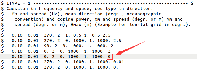
当时间变化时，图像不变，即都为0；

问题：将 case 2 中生成的restart.ww3文件更换为 case 3 中的，再ww3_shel，图像是 case 3 中的吗？

是的~~

结论：运行不是目的，得到相应的.ww3文件才是~~

问题：case 3 不需要restart.ww3，再ww3_shel，可行吗？

可行~

得到的nc文件与 case 3 有 restart.ww3 时一致~~

log.ww3 是否也一致？不一致~~

calm

无restart.ww3时的log.ww3

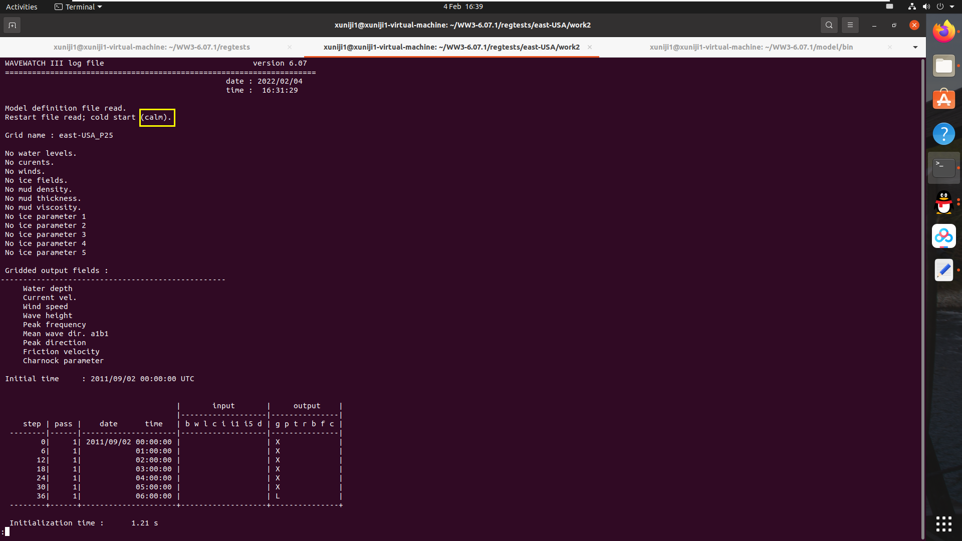
idealized

有restart.ww3时的log.ww3

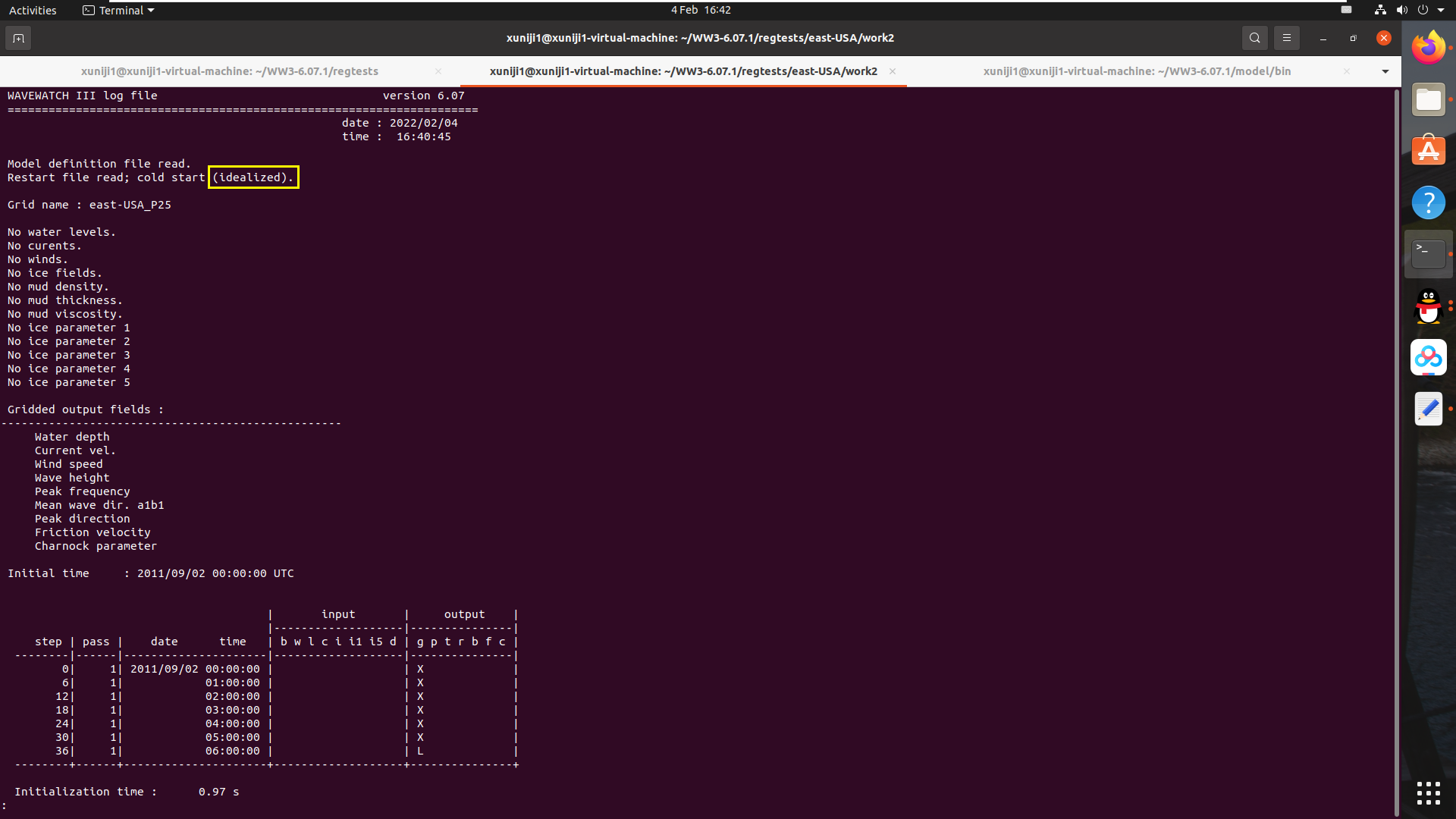
—————————————CCMP风场下运行

参考资料

https://liu-jincan.github.io/2022/01/02/wavewatch3/06-tutorial-inout/

inout教程；

https://data.remss.com/ccmp/

来自于老师；

CCMP介绍中还有ftp；

在regtests的east-USA中，根据执行ww3_prnc的run_test命令，配置相关文件并执行

用 download_ccmp.m从https://data.remss.com/ccmp/获取包含所需时间段的nc文件，放在一个文件夹下；再用 merge_ccmp_ww3.m将这些nc文件合成一个，放进输入文件夹中，重命名为 wind.nc.ccmp01to10，用此风场文件时，cp wind.nc.ccmp01to10 wind.nc。

执行ww3_prnc的run_test命令为：（info中有记录）

cd $regtests
./east-USA/run_test -i input -c Gnu -s Ifremer1 -N -r ww3_prnc -w work3 ../model east-USA

在输入文件夹中创建 ww3_prnc.nml.1，用此文件时 cp ww3_prnc.nml.1 ww3_prnc.nml：

（主要参考inout教程中的，$model中也有）

! -------------------------------------------------------------------- !
! WAVEWATCH III ww3_prnc.nml - Field preprocessor                      !
! -------------------------------------------------------------------- !


! -------------------------------------------------------------------- !
! Define the forcing fields to preprocess via FORCING_NML namelist
!
! * only one FORCING%FIELD can be set at true
! * only one FORCING%grid can be set at true
! * tidal constituents FORCING%tidal is only available on grid%asis with FIELD%level or FIELD%current
!
! * namelist must be terminated with /
! * definitions & defaults:
!     FORCING%TIMESTART            = '19000101 000000'  ! Start date for the forcing field
!     FORCING%TIMESTOP             = '29001231 000000'  ! Stop date for the forcing field
!
!     FORCING%FIELD%ICE_PARAM1     = F           ! Ice thickness                      (1-component)
!     FORCING%FIELD%ICE_PARAM2     = F           ! Ice viscosity                      (1-component)
!     FORCING%FIELD%ICE_PARAM3     = F           ! Ice density                        (1-component)
!     FORCING%FIELD%ICE_PARAM4     = F           ! Ice modulus                        (1-component)
!     FORCING%FIELD%ICE_PARAM5     = F           ! Ice floe mean diameter             (1-component)
!     FORCING%FIELD%MUD_DENSITY    = F           ! Mud density                        (1-component)
!     FORCING%FIELD%MUD_THICKNESS  = F           ! Mud thickness                      (1-component)
!     FORCING%FIELD%MUD_VISCOSITY  = F           ! Mud viscosity                      (1-component)
!     FORCING%FIELD%WATER_LEVELS   = F           ! Level                              (1-component)
!     FORCING%FIELD%CURRENTS       = F           ! Current                            (2-components)
!     FORCING%FIELD%WINDS          = F           ! Wind                               (2-components)
!     FORCING%FIELD%WIND_AST       = F           ! Wind and air-sea temp. dif.        (3-components)
!     FORCING%FIELD%ICE_CONC       = F           ! Ice concentration                  (1-component)
!     FORCING%FIELD%ICE_BERG       = F           ! Icebergs and sea ice concentration (2-components)
!     FORCING%FIELD%DATA_ASSIM     = F           ! Data for assimilation              (1-component)
!
!     FORCING%GRID%ASIS            = F           ! Transfert field 'as is' on the model grid
!     FORCING%GRID%LATLON          = F           ! Define field on regular lat/lon or cartesian grid
!
!     FORCING%TIDAL                = 'unset'     ! Set the tidal constituents [FAST | VFAST | 'M2 S2 N2']
! -------------------------------------------------------------------- !
&FORCING_NML
  FORCING%FIELD%WINDS          = T
  FORCING%GRID%LATLON          = T
/

! -------------------------------------------------------------------- !
! Define the content of the input file via FILE_NML namelist
!
! * input file must respect netCDF format and CF conventions
! * input file must contain :
!      -dimension : time, name expected to be called time
!      -dimension : longitude/latitude, names can defined in the namelist
!      -variable : time defined along time dimension
!      -attribute : time with attributes units written as ISO8601 convention
!      -attribute : time with attributes calendar set to standard as CF convention
!      -variable : longitude defined along longitude dimension
!      -variable : latitude defined along latitude dimension
!      -variable : field defined along time,latitude,longitude dimensions
! * FILE%VAR(I) must be set for each field component
!
! * namelist must be terminated with /
! * definitions & defaults:
!     FILE%FILENAME      = 'unset'           ! relative path input file name
!     FILE%LONGITUDE     = 'unset'           ! longitude/x dimension name
!     FILE%LATITUDE      = 'unset'           ! latitude/y dimension name
!     FILE%VAR(I)        = 'unset'           ! field component
!     FILE%TIMESHIFT     = '00000000 000000' ! shift the time value to 'YYYYMMDD HHMMSS'
! -------------------------------------------------------------------- !
&FILE_NML
  FILE%FILENAME      = 'wind.nc'
  FILE%LONGITUDE     = 'longitude'
  FILE%LATITUDE      = 'latitude'
  FILE%VAR(1)        = 'u10m'
  FILE%VAR(2)        = 'v10m'
/


! -------------------------------------------------------------------- !
! WAVEWATCH III - end of namelist                                      !

! ——————————————————————– !


4. 执行，在输出文件夹得到结果：

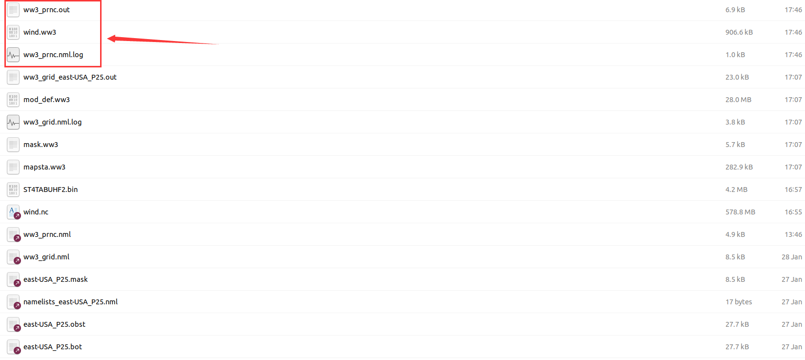
   ![](https://raw.githubusercontent.com/Liu-Jincan/PicGo/main/img/20220210174810.png)

   > 建议把生成的`wind.ww3`文件保存到输入文件夹，`wind.ww3.ccmp01to10`。

## 问题：ww3_prnc，为什么inout教程的wind.nc可以，老师的wind.nc可以，ccmp的不行；

出现的错误：

Program received signal SIGSEGV: Segmentation fault - invalid memory reference.

Backtrace for this error:
#0 0x7f1c8d109d21 in ???
#1 0x7f1c8d108ef5 in ???
#2 0x7f1c8cd4020f in ???
#3 0x7f1c8cab6d95 in ???
#4 0x7f1c8cf507d1 in ???
#5 0x561a038418e6 in ???
#6 0x561a037cd003 in ???
#7 0x561a037ca6b8 in ???
#8 0x7f1c8cd210b2 in ???
#9 0x561a037ca6ed in ???
#10 0xffffffffffffffff in ???
./east-USA/run_test: line 1257: 42224 Segmentation fault (core dumped) $path_e/$prog > $ofile

ERROR: Error occured during /home/xuniji1/WW3-6.07.1/model/exe/ww3_prnc execution




探索发现的问题：（nc文件的format？）

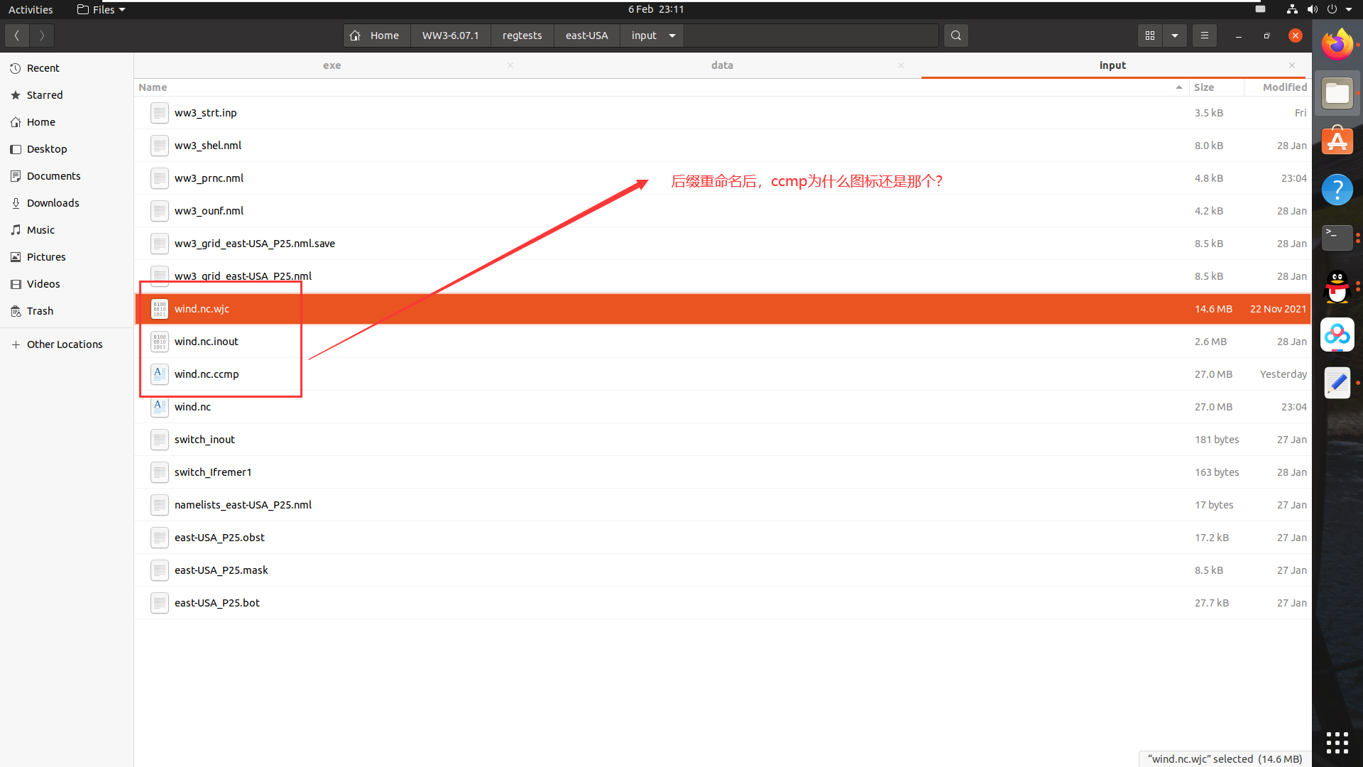
![](https://raw.githubusercontent.com/Liu-Jincan/PicGo/main/img/20220206231221.png)

解决方法可能是 ccmp 的read_routine 教程，生成新的 ccmp 的 nc 文件；（**失败**）

解决办法可能是需要合并 ccmp 的nc文件；（**失败**）

解决办法可能是 nc 文件的format问题，因为inout教程文件都是 `64-bit`，而ccmp的是`class`；（**失败**，老师的也是`class`）

解决办法可能是 nc 文件的变量type问题，因为inout教程和老师的文件都是 `double`，而ccmp的是`single`；（**失败**）

分析，将inout的nc文件，进行`merge_ccmp.m`，能否成功？（**失败**）是内容的问题，还是**merge问题**

netcdf.endDef(cid);
错误使用 netcdflib
NetCDF 库在执行 ‘endDef’ 函数期间遇到错误 - ‘Not a valid data type or _FillValue type mismatch (NC_EBADTYPE)’。


`_FillValue`名称不统一；

尝试`NETCDF4`模式？（失败）

尝试减少没必要的属性？（**成功**）

ww3_prnc.nml 要求

…


完全按照inout教程的：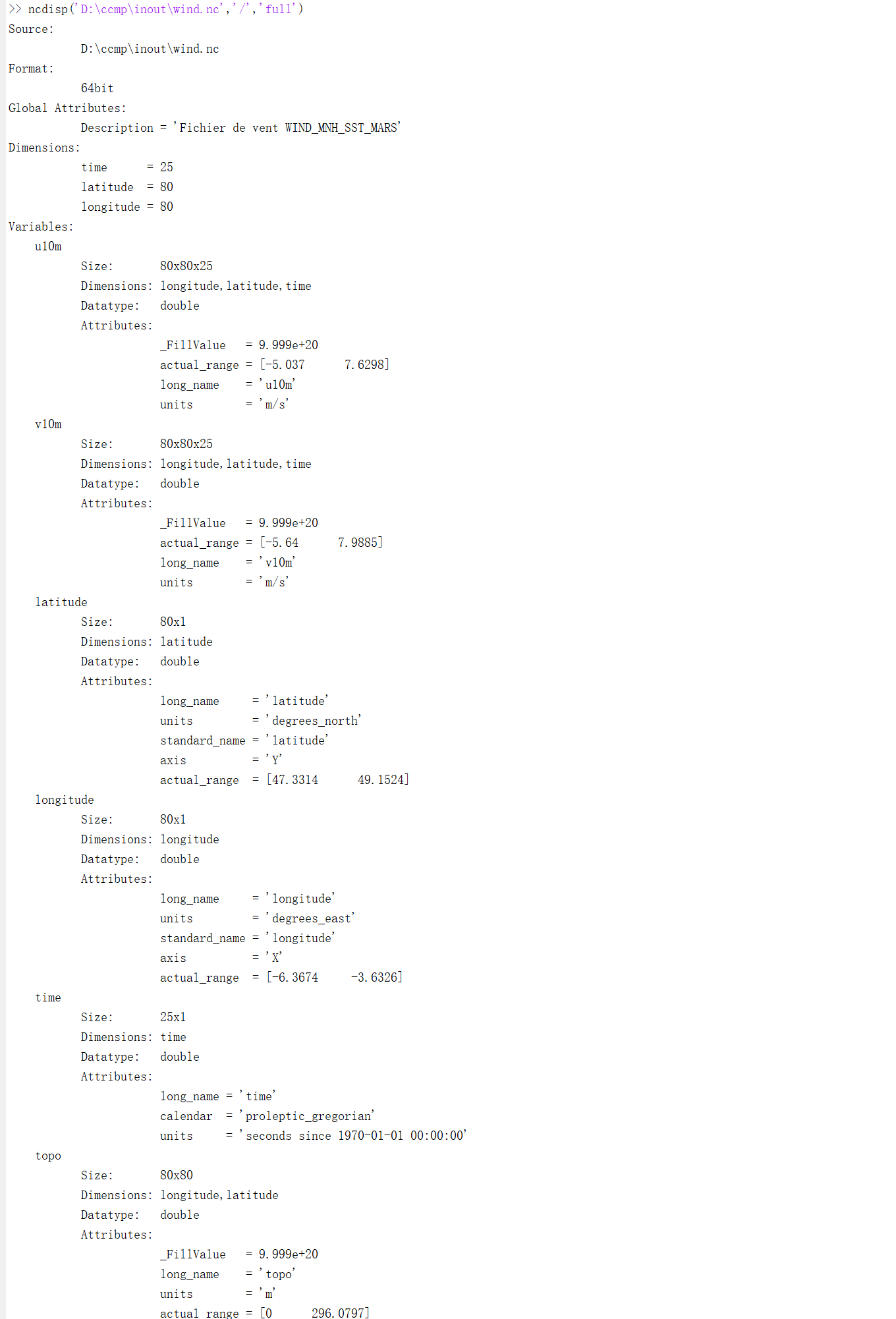

![](https://raw.githubusercontent.com/Liu-Jincan/PicGo/main/img/20220210151514.png)

我的：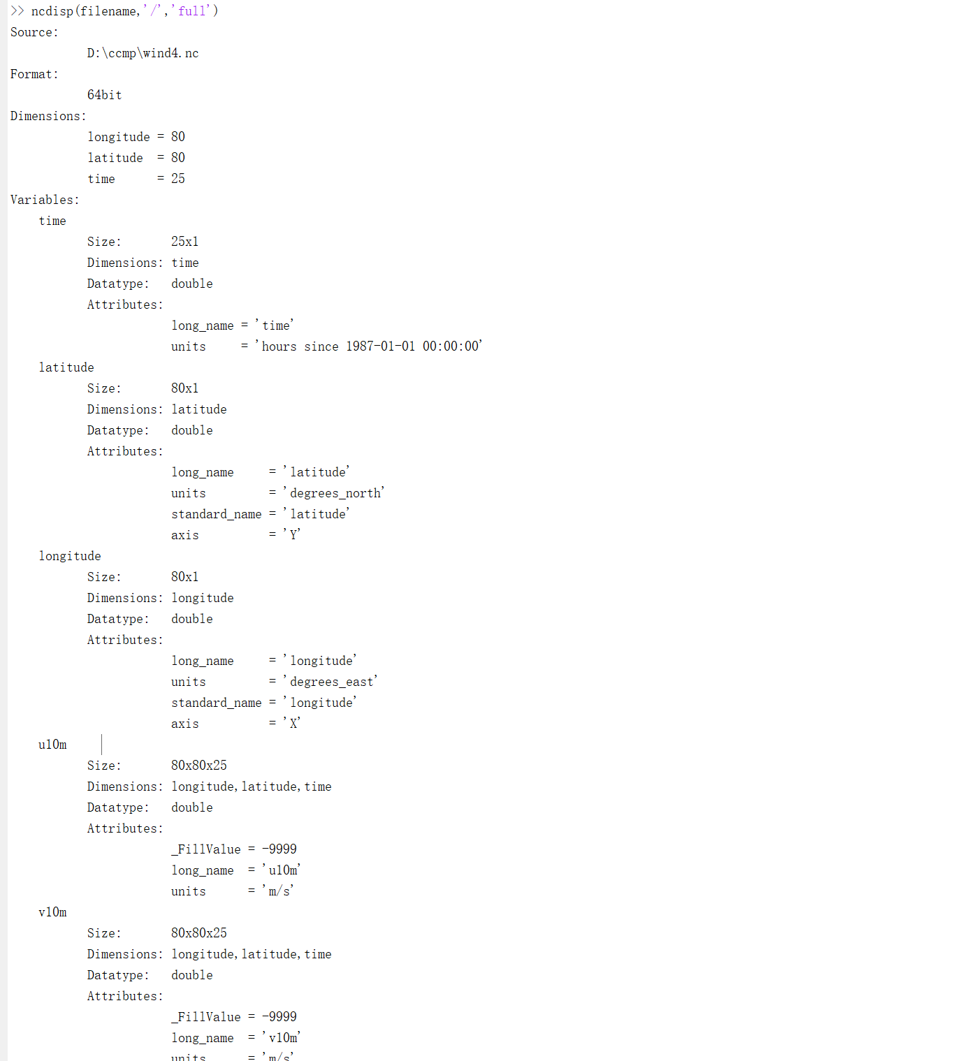

![](https://raw.githubusercontent.com/Liu-Jincan/PicGo/main/img/20220210151642.png)

尝试在ubuntu上建立？

尝试求助大佬？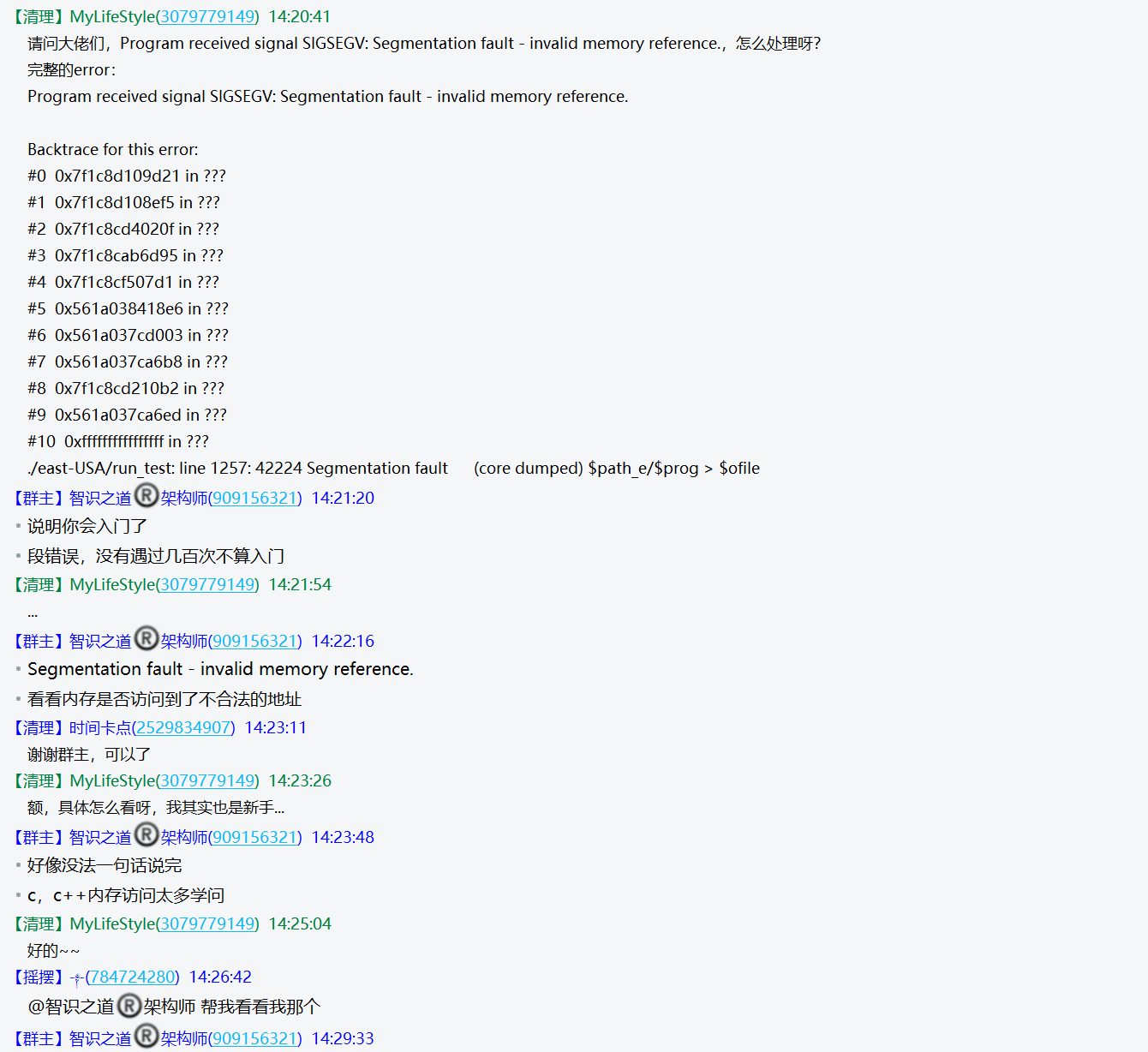

![](https://raw.githubusercontent.com/Liu-Jincan/PicGo/main/img/20220210143504.png)

<img src="https://raw.githubusercontent.com/Liu-Jincan/PicGo/main/img/20220210152001.png" alt=" " style="zoom:80%;" />

分析`inout`教程；

1. ww3_prnc的运行是需要ww3_grid运行的结果`mod_def.ww3`，单独运行ww3_prnc，仍然是那个错误；



## 在regtests的east-USA中，根据执行ww3_shel的run_test命令，配置相关文件并执行

1. 执行ww3_shel的run_test命令为：

  ```bash
  cd $regtests
  ./east-USA/run_test -i input -c Gnu -s Ifremer1 -N -r ww3_shel -w work3 ../model east-USA

在输入文件夹中创建 ww3_shel.nml.***，先采用inout教程中最初始的 ww3_shel.nml模板，然后将风输入的强制标志设置为“外部强制文件(external forcing field)”的 'T'；用此文件时，cp ww3_shel.nml.*** ww3_shel.nml，以下是 ww3_shel.nml.wind：

这里确定时间段（domain 时间、output 时间）~~

! -------------------------------------------------------------------- !
! WAVEWATCH III ww3_shel.nml - single-grid model                       !
! -------------------------------------------------------------------- !


! -------------------------------------------------------------------- !
! Define top-level model parameters via DOMAIN_NML namelist
!
! * IOSTYP defines the output server mode for parallel implementation.
!             0 : No data server processes, direct access output from
!                 each process (requires true parallel file system).
!             1 : No data server process. All output for each type 
!                 performed by process that performs computations too.
!             2 : Last process is reserved for all output, and does no
!                 computing.
!             3 : Multiple dedicated output processes.
!
! * namelist must be terminated with /
! * definitions & defaults:
!     DOMAIN%IOSTYP =  1                 ! Output server type
!     DOMAIN%START  = '19680606 000000'  ! Start date for the entire model 
!     DOMAIN%STOP   = '19680607 000000'  ! Stop date for the entire model
! -------------------------------------------------------------------- !
&DOMAIN_NML
DOMAIN%START   = '20110902 000000'
DOMAIN%STOP    = '20110902 060000'
/

! -------------------------------------------------------------------- !
! Define each forcing via the INPUT_NML namelist
!
! * The FORCING flag can be  : F for "no forcing"
!                              T for "external forcing file"
!                              H for "homogenous forcing input"
!                              C for "coupled forcing field"
!
! * homogeneous forcing is not available for ICE_CONC
!
! * The ASSIM flag can :  F for "no forcing"
!                         T for "external forcing file"
!
! * namelist must be terminated with /
! * definitions & defaults:
!     INPUT%FORCING%WATER_LEVELS  = F
!     INPUT%FORCING%CURRENTS      = F
!     INPUT%FORCING%WINDS         = F
!     INPUT%FORCING%ICE_CONC      = F
!     INPUT%FORCING%ICE_PARAM1    = F
!     INPUT%FORCING%ICE_PARAM2    = F
!     INPUT%FORCING%ICE_PARAM3    = F
!     INPUT%FORCING%ICE_PARAM4    = F
!     INPUT%FORCING%ICE_PARAM5    = F
!     INPUT%FORCING%MUD_DENSITY   = F
!     INPUT%FORCING%MUD_THICKNESS = F
!     INPUT%FORCING%MUD_VISCOSITY = F
!     INPUT%ASSIM%MEAN            = F
!     INPUT%ASSIM%SPEC1D          = F
!     INPUT%ASSIM%SPEC2D          = F
! -------------------------------------------------------------------- !
&INPUT_NML
INPUT%FORCING%WINDS = 'T' 
/

! -------------------------------------------------------------------- !
! Define the output types point parameters via OUTPUT_TYPE_NML namelist
!
! * the point file is a space separated values per line : lon lat 'name'
!
! * the full list of field names is : 
!  DPT CUR WND AST WLV ICE IBG D50 IC1 IC5 HS LM T02 T0M1 T01 FP DIR SPR
!  DP HIG EF TH1M STH1M TH2M STH2M WN PHS PTP PLP PDIR PSPR PWS TWS PNR
!  UST CHA CGE FAW TAW TWA WCC WCF WCH WCM SXY TWO BHD FOC TUS USS P2S
!  USF P2L TWI FIC ABR UBR BED FBB TBB MSS MSC DTD FC CFX CFD CFK U1 U2 
!
! * output track file formatted (T) or unformated (F)
!
! * coupling fields exchanged list is :
!   - Sent fields by ww3:
!       - Ocean model : T0M1 OCHA OHS DIR BHD TWO UBR FOC TAW TUS USS LM DRY
!       - Atmospheric model : ACHA AHS TP (or FP) FWS
!       - Ice model : IC5 TWI
!   - Received fields by ww3:
!       - Ocean model : SSH CUR
!       - Atmospheric model : WND
!       - Ice model : ICE IC1 IC5
!
! * namelist must be terminated with /
! * definitions & defaults:
!     TYPE%FIELD%LIST         =  'unset'
!     TYPE%POINT%FILE         =  'points.list'
!     TYPE%TRACK%FORMAT       =  T
!     TYPE%PARTITION%X0       =  0
!     TYPE%PARTITION%XN       =  0
!     TYPE%PARTITION%NX       =  0
!     TYPE%PARTITION%Y0       =  0
!     TYPE%PARTITION%YN       =  0
!     TYPE%PARTITION%NY       =  0
!     TYPE%PARTITION%FORMAT   =  T
!     TYPE%COUPLING%SENT      = 'unset'
!     TYPE%COUPLING%RECEIVED  = 'unset'
!
! -------------------------------------------------------------------- !
&OUTPUT_TYPE_NML
TYPE%FIELD%LIST          = 'HS FP DIR DP CHA UST DPT CUR WND'
/

! -------------------------------------------------------------------- !
! Define output dates via OUTPUT_DATE_NML namelist
!
! * start and stop times are with format 'yyyymmdd hhmmss'
! * if time stride is equal '0', then output is disabled
! * time stride is given in seconds
!
! * namelist must be terminated with /
! * definitions & defaults:
!     DATE%FIELD%START         =  '19680606 000000'
!     DATE%FIELD%STRIDE        =  '0'
!     DATE%FIELD%STOP          =  '19680607 000000'
!     DATE%POINT%START         =  '19680606 000000'
!     DATE%POINT%STRIDE        =  '0'
!     DATE%POINT%STOP          =  '19680607 000000'
!     DATE%TRACK%START         =  '19680606 000000'
!     DATE%TRACK%STRIDE        =  '0'
!     DATE%TRACK%STOP          =  '19680607 000000'
!     DATE%RESTART%START       =  '19680606 000000'
!     DATE%RESTART%STRIDE      =  '0'
!     DATE%RESTART%STOP        =  '19680607 000000'
!     DATE%BOUNDARY%START      =  '19680606 000000'
!     DATE%BOUNDARY%STRIDE     =  '0'
!     DATE%BOUNDARY%STOP       =  '19680607 000000'
!     DATE%PARTITION%START     =  '19680606 000000'
!     DATE%PARTITION%STRIDE    =  '0'
!     DATE%PARTITION%STOP      =  '19680607 000000'
!     DATE%COUPLING%START      =  '19680606 000000'
!     DATE%COUPLING%STRIDE     =  '0'
!     DATE%COUPLING%STOP       =  '19680607 000000'
!
!     DATE%RESTART             =  '19680606 000000' '0' '19680607 000000'
! -------------------------------------------------------------------- !
&OUTPUT_DATE_NML
DATE%FIELD          = '20110902 000000' '3600' '20110902 060000'
/

! -------------------------------------------------------------------- !
! Define homogeneous input via HOMOG_COUNT_NML and HOMOG_INPUT_NML namelist
!
! * the number of each homogeneous input is defined by HOMOG_COUNT
! * the total number of homogeneous input is automatically calculated
! * the homogeneous input must start from index 1 to N
! * if VALUE1 is equal 0, then the homogeneous input is desactivated
! * NAME can be IC1, IC2, IC3, IC4, IC5, MDN, MTH, MVS, LEV, CUR, WND, ICE, MOV
! * each homogeneous input is defined over a maximum of 3 values detailled below :
!     - IC1 is defined by thickness
!     - IC2 is defined by viscosity
!     - IC3 is defined by density
!     - IC4 is defined by modulus
!     - IC5 is defined by floe diameter
!     - MDN is defined by density
!     - MTH is defined by thickness
!     - MVS is defined by viscosity
!     - LEV is defined by height
!     - CUR is defined by speed and direction
!     - WND is defined by speed, direction and airseatemp
!     - ICE is defined by concentration
!     - MOV is defined by speed and direction
!
! * namelist must be terminated with /
! * definitions & defaults:
!     HOMOG_COUNT%N_IC1            =  0
!     HOMOG_COUNT%N_IC2            =  0
!     HOMOG_COUNT%N_IC3            =  0
!     HOMOG_COUNT%N_IC4            =  0
!     HOMOG_COUNT%N_IC5            =  0
!     HOMOG_COUNT%N_MDN            =  0
!     HOMOG_COUNT%N_MTH            =  0
!     HOMOG_COUNT%N_MVS            =  0
!     HOMOG_COUNT%N_LEV            =  0
!     HOMOG_COUNT%N_CUR            =  0
!     HOMOG_COUNT%N_WND            =  0
!     HOMOG_COUNT%N_ICE            =  0
!     HOMOG_COUNT%N_MOV            =  0
!
!     HOMOG_INPUT(I)%NAME           =  'unset'
!     HOMOG_INPUT(I)%DATE           =  '19680606 000000'
!     HOMOG_INPUT(I)%VALUE1         =  0
!     HOMOG_INPUT(I)%VALUE2         =  0
!     HOMOG_INPUT(I)%VALUE3         =  0
! -------------------------------------------------------------------- !
&HOMOG_COUNT_NML
/

&HOMOG_INPUT_NML
/


! -------------------------------------------------------------------- !
! WAVEWATCH III - end of namelist                                      !
! -------------------------------------------------------------------- !

执行，在输出文件夹得到结果：

在regtests的east-USA中，根据执行ww3_ounf的run_test命令，配置相关文件并执行

执行ww3_ounf的run_test命令为：

cd $regtests
./east-USA/run_test -i input -c Gnu -s Ifremer1 -N -r ww3_ounf -w work3 -o netcdf ../model east-USA

在输入文件夹中创建 ww3_ounf.nml.2，用此文件时，cp ww3_ounf.nml.2 ww3_ounf.nml：

先采用inout教程中的 ww3_ounf.nml;

这里需要确定时间（FIELD的时间），不是很懂这里的设置；

! -------------------------------------------------------------------- !
! WAVEWATCH III ww3_ounf.nml - Grid output post-processing             !
! -------------------------------------------------------------------- !

! -------------------------------------------------------------------- !
! Define the output fields to postprocess via FIELD_NML namelist
!
! * the full list of field names FIELD%LIST is : 
!  DPT CUR WND AST WLV ICE IBG D50 IC1 IC5 HS LM T02 T0M1 T01 FP DIR SPR
!  DP HIG EF TH1M STH1M TH2M STH2M WN PHS PTP PLP PDIR PSPR PWS TWS PNR
!  UST CHA CGE FAW TAW TWA WCC WCF WCH WCM SXY TWO BHD FOC TUS USS P2S
!  USF P2L TWI FIC ABR UBR BED FBB TBB MSS MSC DTD FC CFX CFD CFK U1 U2 
!
! * namelist must be terminated with /
! * definitions & defaults:
!     FIELD%TIMESTART            = '19000101 000000'  ! Stop date for the output field
!     FIELD%TIMESTRIDE           = '0'                ! Time stride for the output field
!     FIELD%TIMESTOP             = '29001231 000000'  ! Stop date for the output field
!     FIELD%TIMECOUNT            = '1000000000'       ! Number of time steps
!     FIELD%TIMESPLIT            = 6                  ! [4(yearly),6(monthly),8(daily),10(hourly)]
!     FIELD%LIST                 = 'unset'            ! List of output fields
!     FIELD%PARTITION            = '0 1 2 3'          ! List of wave partitions ['0 1 2 3 4 5']
!     FIELD%SAMEFILE             = T                  ! All the variables in the same file [T|F]
!     FIELD%TYPE                 = 3                  ! [2 = SHORT, 3 = it depends , 4 = REAL]
! -------------------------------------------------------------------- !
&FIELD_NML
  FIELD%TIMESTART        =  '20080310 000000'
  FIELD%TIMESTRIDE       =  '180'
  FIELD%TIMECOUNT        =  '100'
  FIELD%LIST             =  'HS FP DIR DP CHA UST DPT CUR WND'
  FIELD%PARTITION        =  '0'
/

! -------------------------------------------------------------------- !
! Define the content of the input file via FILE_NML namelist
!
! * namelist must be terminated with /
! * definitions & defaults:
!     FILE%PREFIX        = 'ww3.'            ! Prefix for output file name
!     FILE%NETCDF        = 3                 ! Netcdf version [3|4]
!     FILE%IX0           = 1                 ! First X-axis or node index
!     FILE%IXN           = 1000000000        ! Last X-axis or node index
!     FILE%IY0           = 1                 ! First Y-axis index
!     FILE%IYN           = 1000000000        ! Last Y-axis index
! -------------------------------------------------------------------- !
&FILE_NML
/


! -------------------------------------------------------------------- !
! Define the content of the output file via SMC_NML namelist
!
! * For SMC grids, IX0, IXN, IY0 and IYN from FILE_NML are not used.
!   Two types of output are available:
! *   TYPE=1: Flat 1D "seapoint" array of grid cells.
! *   TYPE=2: Re-gridded regular grid with cell sizes being an integer
! *           multiple of the smallest SMC grid cells size.
!
! * Note that the first/last longitudes and latitudes will be adjusted
!  to snap to the underlying SMC grid edges. CELFAC is only used for
!  type 2 output and defines the output cell sizes as an integer
!  multiple of the smallest SMC Grid cell size. CELFAC should be a
!  power of 2, e.g: 1,2,4,8,16, etc...
!
! * namelist must be terminated with /
! * definitions & defaults:
!     SMC%TYPE          = 1              ! SMC Grid type (1 or 2)
!     SMC%SXO           = -999.9         ! First longitude
!     SMC%EXO           = -999.9         ! Last longitude
!     SMC%SYO           = -999.9         ! First latitude
!     SMC%EYO           = -999.9         ! Last latitude
!     SMC%CELFAC        = 1              ! Cell size factor (SMCTYPE=2 only)
!     SMC%NOVAL         = UNDEF          ! Fill value for wet cells with no data
! -------------------------------------------------------------------- !
&SMC_NML
/

! -------------------------------------------------------------------- !
! WAVEWATCH III - end of namelist                                      !
! -------------------------------------------------------------------- !

执行，在输出文件夹得到结果：
ncview可视化nc文件：

ncview ww3.201109.nc，查看Hs。

了解ww3_shel.nml和ww3_ounf参数

case 1：更长的时间段

‘20110831 200000’到’20110911 000000’时间段 ww3_shel.nml 的设置：

&DOMAIN_NML
DOMAIN%START   = '20110831 200000'
DOMAIN%STOP    = '20110911 000000'
/

&OUTPUT_DATE_NML
DATE%FIELD          = '20110831 200000' '3600' '20110911 000000'
/

这个时间段内包含了风场的时间段，但也包含了没有风场的时间段；

ww3_shel运行的全局时间步长，即经过多少时间间隔输出一次，与 ww3_grid.nml的 TIMESTEPS_NML相关：
&TIMESTEPS_NML
  TIMESTEPS%DTMAX         =   600.
  TIMESTEPS%DTXY          =   200.
  TIMESTEPS%DTKTH         =   300.
  TIMESTEPS%DTMIN         =   10.
/
这严重影响着运行时间的长短？待深入了解！

‘20110831 200000’到’20110911 000000’时间段 ww3_ounf.nml 的设置:

&FIELD_NML
  FIELD%LIST             =  'HS FP DIR DP CHA UST DPT CUR WND'
  FIELD%PARTITION        =  '0'
  FIELD%TIMESTRIDE       =  '3600'
  FIELD%TIMESPLIT            = 4
/

&FIELD_NML
  FIELD%LIST             =  'HS FP DIR DP CHA UST DPT CUR WND'
  FIELD%PARTITION        =  '0'
/
这么设置会一直不动，因为 FIELD%TIMESTRIDE = '0' 。

&FIELD_NML
  FIELD%LIST             =  'HS FP DIR DP CHA UST DPT CUR WND'
  FIELD%PARTITION        =  '0'
  FIELD%TIMESTRIDE       =  '180'
/
每一步跨越180s（3分钟），从’19000101 000000’开始，有’1000000000’步，运行时间需要等个1分钟，可以根据 ww3_shel.nml按3600s（1小时）输出，将TIMESTRIDE设置成 3600，运行很快；

这样会生成两个月份的nc文件，ww3.201108.nc和 ww3.201109.nc，调整 FIELD%TIMESPLIT = 4 会按年份输出；

不懂 FIELD%PARTITION = '0'，但好像没什么影响…；

生成了 ww3.2011.nc文件，对其进行 ncview：

发现 hs在没有实际风场的时间段’20110831 200000’到’20110901 000000’也有波高，原因是模式在这个时间段有默认假设的风场，即’20110901 000000’的实际风场，可通过查看 uwnd和 vwnd变量得到模式风场的信息。实际应用中，应在ww3_shel.nml将起始时间和终止时间与风场对应？；
发现模式输出的 uwnd和 vwnd是按每小时输出的，与实际风场信息每6个小时输出不一样；（模式输出的每6小时风场信息和ccmp风场信息一样吗？）

—————————————

给老师的反馈：2022-02-18

老师，根据您2022-01-17号的指导，这个寒假我主要做的内容如下：

了解CCMP风场数据，能实现对CCMP v.2 每天数据的批量爬取，整合成一个nc文件，供ww3_prnc使用；
了解ndbc浮标数据，能实现对特定区域的浮标数据进行批量爬取，匹配nc文件中网格点数据，计算RMSE、BIAS、R、SI，简单画出时序图、散点图，过程中的所有浮标相关的数据都存到matlab的一个table类型变量中；
具体在ww3试验中，选择区域为75°W-58°W、36°N-46°N，分辨率为0.25°，加入了20110901-20110910时间段的CCMP风场数据，运行生成的ww3.2011.nc文件与ncdb的浮标数据进行了对比，整体趋势接近；

所有内容在https://liu-jincan.github.io/2022/01/17/wavewatch3/07-gei-ding-qu-yu-ww3-shi-yan-2022-han-jia-an-pai/上都有记录（打开可能图片会显示的比较慢）；

下一步准备学习同化，将同化部分接入到ww3中。

Jincan

https://Liu-Jincan.github.io/2022/01/17/yan-jiu-sheng-justtry-target/yan-yi-shang-han-jia-gei-ding-qu-yu-ww3-shi-yan-2022-han-jia-an-pai/

All articles in this blog are used except for special statements CC BY 4.0 reprint policy. If reproduced, please indicate source Jincan !

No tag

01-VMware安装+ubuntu虚拟机及其扩容

2022-01-24 VMware

02-VScode搭建C/C++

2022-01-16 VScode编辑器

07-east-USA区域WW3试验（2022寒假安排）

<center>07-给定区域WW3试验（2022寒假安排）</center>

文档托管

—————————————CCMP

参考资料

CCMP Wind Vector Analysis Product (2022-01-17)

Version 2 CCMP Wind Product

Introduction

Product Development

CCMP VERSION-2 UPDATES

Data Product Format

MISSING DATA

Read Routines / Data Access

Browse Images / Graphic Maps

Product Details

Known Issues / Data Caveats

Related Data

References

How to Cite These Data

DATA SET CITATION

JOURNAL REFERENCE

参考资料

下载CCMP数据（matlab, urlwrite 函数）

参考资料

合并CCMP的nc数据（matlab）

合并CCMP的nc数据（matlab，专门用于ww3_prnc）

—————————————

参考资料

Measurement Descriptions and Units（released in 20220211）：包含实时和历史数据文件中各变量的描述

Real Time files & Historical files

General

help topic: Do NDBC’s meteorological and oceanographic sensors measure data for the entire hour?

changes page: Important NDBC Web Site Changes

Station Identifier: How are the station ID numbers created?

data inventory summary: Data Availability Summary for NDBC Platforms

Important Notice to Mariners: NATIONAL WEATHER SERVICE SEEKS COOPERATION TO SAFEGUARD CRITICAL DATA BUOYS

Standard Meteorological Data

Derived Met Values

Supplemental Measurements Data

Continuous Winds

Detailed Wave Summary (Realtime data files only)

Spectral Wave Data

Ocean Current Data

Ocean Current Data (Expanded ADCP format)

Marsh-McBirney Current Measurements

Water Level

Oceanographic Data

Solar Radiation Data

DART (Tsunameters) Measurements

24-Hour Rain Measurements

Hourly Rain Measurements

10-Minute Rain Measurements

Housekeeping Measurements

Discontinued Measurement Abbreviations

参考资料

How can I configure MATLAB to allow access to self-signed HTTPS servers?

question description

answer：MathWorks Support Team, STAFF, 2019-6-19

answer：Jerome Blaha，2021-7-26

answer：Chirag Patel，2017-3-9，（成功~~）

下载、plot NDBC浮标Standard Meterological历史数据（matlab）

ndbc_station_info.m

如何查看火狐浏览器的useragent

如何为MATLAB配置ndbc的 HTTPS servers的证书（Certificate）？

matlab 如何储存大量数据比较合理？

MATLAB如何使用table函数创建和编辑表格？

second, function, path_save

ndbc_station_info_needed.m

second, function, path_save

ndbc_station_info_needed_plot.m

南海论文中浮标的图

second, function, path_save

ndbc_station_info_needed_etopo1.m

second, function, path_save

etopo1来源机构及其论文参考

ndbc_station_download.m

问题得到大佬们的指点解决：str2num()

ndbc 数据不同年份的数据格式

ndbc_station_download.m（第二版本, 使用 datetime 数据类型 ）

third, ndbc_station_download_NC_analyse

`<center>`07-给定区域WW3试验（2022寒假安排）`</center>`

ndbc_station_download.m（第二版本, 使用 datetime 数据类型）