<center>07-阅读:使用循环神经网络进行数据同化的观测误差协方差规范-2021 </center>
参考资料
英文名:Observation error covariance specification in dynamical systems for data assimilation using recurrent neural networks
期刊:《Neural Computing and Applications》,LetPub,https://www.letpub.com.cn/index.php?page=journalapp&view=search
这个期刊好像不错~~
作者:Sibo Cheng, Mingming Qiu
来自于Wjc老师的分享,用于2022创新基金的思考的出发点;
谷歌浏览器无法阅读的公式,火狐浏览器可以~~~😎,但是翻译质量没有谷歌翻译好┭┮﹏┭┮思维流记录更好吧~
Abstract
Data assimilation techniques are widely used to predict complex dynamical systems with uncertainties, based on timeseries observation data. Error covariance matrices modeling is an important element in data assimilation algorithms which can considerably impact the forecasting accuracy. The estimation of these covariances, which usually relies on empirical assumptions and physical constraints, is often imprecise and computationally expensive, especially for systems of large dimensions. In this work, we propose a data-driven approach based on long short term memory (LSTM) recurrent neural networks (RNN) to improve both the accuracy and the efficiency of observation covariance specification in data assimilation for dynamical systems.
误差协方差矩阵建模是数据同化算法中的一个重要元素,它会极大地影响预测的准确性。这些协方差的估计通常依赖于经验假设和物理约束,通常不精确且计算成本很高,尤其是对于大尺寸系统。
Learning the covariance matrix from observed/simulated time-series data, the proposed approach does not require any knowledge or assumption about prior error distribution, unlike classical posterior tuning methods.
与经典的后验调整方法不同,所提出的方法不需要任何关于先验误差分布的知识或假设。
We have compared the novel approach with two state-of-the-art covariance tuning algorithms, namely DI01 and D05, first in a Lorenz dynamical system and then in a 2D shallow water twin experiments framework with different covariance parameterization using ensemble assimilation.
两种最先进的协方差调整算法(即 DI01 和 D05)Lorenz 动力系统二维浅水孪生实验
This novel method shows significant advantages in observation covariance specification, assimilation accuracy, and computational efficiency.
新方法在观测协方差规范、同化精度和计算效率方面具有显着优势。
Acknowledgments
S.Cheng would like to thank Dr. D.Lucor, Dr. J-P.Argaud, Dr. B.Iooss, and Dr. A.Ponc¸ot for fruitful discussions about the error covariance computation. This research was supported by EDF R&D. This research was partially funded by the Leverhulme Centre for Wildfires, Environment and Society through the Leverhulme Trust, grant number RC-2018-023.
Declarations (with code)
Conflict of interest statement
…
Code availability
Code for the proposed LSTM-based covariance specification, together with DI01, D05 methods, for both Lorenz and shallow water models is available at https://github.com/scheng1992/ LSTM_Covariance.
Contribution statement
…
Open Access
…
9 Discussion
The precision of DA reconstruction/prediction depends heavily on the specification of both the background and the observation error correlation. The latter is often challenging to estimate in real-world applications because of the dynamic nature of the observation data. Furthermore, the observation matrix $\mathbf{R}$ can not be empirically estimated from an ensemble of simulated trajectories, unlike the background error covariance. In this paper, we review in detail some well-known observation covariance tuning algorithms [23, 54], based on time-variant posterior innovation quantities. These methods, being widely adopted in geoscience, rely on some specific prior assumptions such as knowledge of the correlation structure [23] or the background matrix [24]. This is difficult to fulfill in some domains where very little knowledge about the prior error is available.
为什么?:观察矩阵 R 与背景误差协方差不同,不能从模拟轨迹的集合中凭经验估计什么是?:时变后验创新量
In this study, we have proposed a novel machine learning approach based on LSTM neural networks to predict the $\mathbf{R}$ matrix using time series observation data as model input. Similar to the work of [23, 24], $\mathbf{R}$ is assumed to be time-invariant, at least over a sufficiently long time period. Both the Kalman- and variational-type assimilation methods can benefit from the method proposed in this paper for improving the assimilation accuracy. The proposed data-driven approach also contributes to tackling one of the major bottlenecks of DA: it is time-consuming and computationally expensive to update covariance matrix, by mapping raw sensor observations to observation error covariance matrix. In both the Lorenz96 and the shallow water models presented in this paper, the LSTM-based approach displays significant strength, compared to classical posterior tuning methods DI01 and D05, in terms of:
- (i) estimation accuracy of the observation covariance $\mathbf{R}$;
- (ii) reconstruction and prediction accuracy of the DA schema, using the estimated $\mathbf{R}$ matrix;
- (iii) computational efficiency of the online covariance estimation;
- (iv) flexibility of different model parameterization. It is worth mentioning that an important limitation of the proposed LSTM-based method is the specification of $\Phi_{\mathbf{R}}$ which defines the range of parameters for training.
-> 很强大,可以做很多这方面的工作
Since we assume that the observation matrix is timeinvariant, the proposed approach could only deal with fixed sensor placement for dynamical systems, which is also the case of DI01 and D05 tuning algorithms. The possibility of time-variant sensor placement warrants further investigation. As pointed out by [55], the DL model can be stolen or reverse engineered, by model inversion or model extraction attack. Despite the fact that all data used in the current study is generated from toy models, it is important to ensure the data privacy when applying the model to real applications.
限制只能在空间点上进行?:只能处理动态系统的固定传感器放置
Future research should also consider applying the new method to a broader range of real-world problems, including NWP, hydrology, and object tracking, where the offline data simulation could be more computationally expensive compared to the two test models presented in this paper. To this end, future studies could also investigate the combination of model reduction methods, such as domain localization [56], proper orthogonal decomposition, information-based data compression [57], auto-encoder neural networks [58], and the current covariance estimation method. More precisely, the data assimilation can be performed in the compressed low dimensional space (e.g., obtained from POD or auto-encoder). The LSTM-based covariance specification algorithm developed in this work can be used to estimate the observation error covariance matrices in the low dimensional space for improving the accuracy of reduced-order data assimilation approaches.
更广泛的现实问题创新工作:为了减少计算成本,压缩的低维空间
1 Introduction
In order to improve the reconstruction and prediction of dynamical systems with uncertainties, data assimilation (DA) techniques, originally developed in numerical weather prediction (NWP) [1] and geosciences [2], are widely applied to industrial problems, such as hydrology [3], wildfire forecasting [4], drought monitoring[5] and nuclear engineering [6].
DA algorithms aim to find the optimal approximation (also known as the analyzed state) of the state variables (usually representing a physical field of interest, such as velocity, temperature, etc.,), relying on prior estimations and real-time observations, both assumed to be noisy. Due to the large dimension (often ranging from $10^6$ to $10^{10}$ in NWP and geoscience problems), prior errors are supposed to be Gaussian distributed for the sake of simplicity [7]. As a consequence, the prior error distribution can be perfectly characterized by the first (mean) and the second (covariance) moment.
DA算法:改进具有不确定性的动力系统的重建和预测,依靠先前的估计和实时观察来找到状态变量,为了简单起见,先验误差应该是高斯分布的The output of the DA algorithms is determined through some optimization function where the weight of prior simulations and observations is determined by the associated error covariance matrices, respectively named as background and observation covariances.
解释了DA中误差协方差矩阵的实质:模拟和观察的权重由相关的误差协方差矩阵确定,分别称为背景和观察协方差。These error covariance matrices thus provide crucial information in DA algorithms [8], for not only the estimation of the analyzed state but also specifying posterior error distributions [9].
DA中误差协方差矩阵的意义:不仅用于估计分析状态,还用于指定后验误差分布The prior errors represented by these matrices, especially in the case of observation errors, consisting of an ensemble of different sources of noise/uncertainties, including model error, instrument noise, and representativity error [10, 11].
用矩阵表示的先验误差包含哪些:模型误差、仪器噪声和代表性误差
In statistics, the covariance matrix of a random vector is often obtained via empirical estimation where a sufficient number of simultaneous samplings is required to avoid estimation bias [12]. Moreover, when the sampling number is inferior to the problem dimension, the estimated covariance will be rank deficient. In DA problems, the high dimensionality and lack of simultaneous data (i.e., several backgrounds or observation trajectories in the same time window) represent significant obstacles of covariance computation in data assimilation [13].
DA中协方差计算的重大障碍:高维和缺乏同时数据
To overcome these difficulties, we often rely on calibration (e.g., least-square) methods based on some generic correlation kernels, often with homogeneous and isotropic characteristics [14].
- Balanced operators can be employed for multivariate systems [15].
- In terms of correlation kernels, the family of Matérn functions, including the Exponential kernel (Matérn 1/2), the Balgovind kernel (Matérn 3/2, also known as second-order auto-regressive (SOAR) function), and the Gaussian kernel (Matérn 5/2), is often prioritized for covariance computing owing to its smoothness and capability to capture spatial correlations in physical processes [10, 16, 17].
- Other stationary covariance models involve, for instance, convolution formulation [18] or diffusion-based operators [19], both contribute to an efficient storage of the covariance matrices. However, limited by homogeneous and isotropic assumptions, it remains cumbersome to represent complex spatial correlation (often multi-dimensional and multivariate) using these one-dimensional kernels.
解决DA中协方差计算重大障碍的经典方法
In this study, we develop and test a novel data-driven approach based on recurrent neural networks (RNNs) to improve both the accuracy and the efficiency of observation covariance specification in dynamical data assimilation problems. The novel approach is tested and compared with two state-of-the-art covariance tuning algorithms in two different digital experiments with parametric and nonparametric covariance estimation, respectively.
本文创新点~,新的方法,进行同化协方差的计算~
The paper is organized as follows. In Section 2, we introduce the related work for error covariance specification. The problem statement and the contribution of this paper are described in Section 3. Data assimilation techniques and the ensemble methods are introduced briefly in Section 4. We then describe traditional posterior covariance tuning algorithms DI01 and D05 in Section 5. The novel LSTM-based method is introduced in Section 6, followed by the comparison in the Lorenz (Section 7) and the shallow water twin experiments (Section 8). We close the paper with a discussion in Section 9.
2 Related work
To gain a clearer insight into covariance evolution,
some ensemble-based methods such as [1] (NMC) and [20] (EnKF), have been developed to provide a non-parametric covariance estimation. These methods depend on the propagation of an ensemble of simulated trajectories, initialized either at different forecasting time steps (NMC) or by adding some artificially set perturbations to the current state (EnKF). These methods are more appropriate for modeling the background matrix compared rather than the observation matrix. The latter, independent from the numerical simulations, can not be represented by the propagation of artificially added noises.
The Particle-Aided Unscented Kalman Filter [21] can estimate systems with high nonlinearity with a real-time updating of the background matrix. However, the observation matrix can not be estimated directly via the Particle-Aided Unscented Kalman Filter.
上面两点说明,NFC,EnKF,PAUKF,这些方法是适用于背景误差协方差的,不适用于观测误差协方差。In practice, the observation matrix is often set to be diagonal or spatially isotropic for the sake of simplicity (e.g. [22]). However, it is shown in the work of [10] that well-specified correlated observation covariances can significantly improve the performance of DA algorithms.
这一点说明,简单的观测误差协方差是不够好的。
Several methods of data-derived posterior diagnosis have also been developed based on the analysis of innovation quantities.(The innovation quantities consist of the difference between the observations and the projected background/analyzed state in the observation space).
innovation quantities,应该是个专有名称,可能不叫创新量,可能可以在同化课程那个pdf笔记中找到相关的介绍
As a strong contributor to this topic, the meteorology community developed several well-known posterior diagnoses and their improved versions [23–25] to adjust the background/observation ratio, the correlation scale length, or the full covariance structure in the observation space (both the observation matrix and the projected background matrix).
Some iterative processes [26, 27] based on the fixed-point theory have also been proposed for error covariance tuning.
Recent works of [28, 29] have proved the convergence of so-called Desroziers iterative methods[24] (also known as D05) in the ideal case. In brief, they have mathematically proved that, by using a semi-positive definite matrix as an initial guess, D05 iterative method converges on the exact time-invariant (at least over a sufficiently long time period) observation error covariance, when the background matrix and the transformation operator (which maps the state variables to real-time observations) are perfectly known a priori. (Here, by the term ‘‘exact’’, we refer to the covariance truly corresponding to the remaining errors present in the observation space).
On the other hand, it is also mentioned by [29] that a regularization step is necessary for practice for applying D05 and the convergence of the regularized iterations remains an open question [3, 29].
To deal with timevarying systems, lag-innovation statistics are used for error covariance estimation [30]. The essential idea is to build a secondary Kalman-filtering process for adjusting error covariances using time-shifted innovation vectors.
For more details of the innovation-based methods, we refer to the overview of [13] which also covers some other estimation methods, such as the family of likelihood-based approaches and expectation-maximum(EM) methods.
3 Problem statement and contribution (Q)
Our work lies in a similar condition of [24, 29] where both the state forward model and the transformation operator are presumed to be well known.
↑ 前向模型,应该是动力模式,本文是M的斜体加粗
↑ 转换算子,应该是观测算子,本文是H的斜体,线性是H
As the main difficulty concerns the non-synchronous time-variant observations in dynamical systems (which prevents empirical estimation), in this work we propose the use of recurrent neural networks (RNNs) [31] for the specification of the observation matrix across the underlying dynamics of the observed quantities.
RNN has been widely adapted for the prediction/reconstruction of dynamical systems, especially in natural language processing (NLP) [32] and image/video processing [33] due to its convincing capacity for dealing with time series. More recently, RNN has also made their way to other engineering fields such as biomedical applications and computational fluid mechanics [34].
↑ RNN 的优点,广泛被应用In general, the combination of deep learning and data assimilation methods [35, 36] has been widely adapted and analyzed in a variety of industrial applications, including air pollution [37] and ocean-atmosphere modeling [38].
A convolutional neural network (CNN) for covariance estimation has also been suggested in the work of [39].
In this study, we propose a novel methodology for LSTM-based covariance estimation which can be easily integrated into any DA schema for dynamical systems.
Q:↑ 新方法,真的很容易用进去吗?~Here, we first construct a set of training covariance matrices, being either parametric or non-parametric, within a certain range defined a priori. For each matrix in the training set, we then simulate a dynamic trajectory of the observation vector relying on the knowledge of the forward model where the noises at each time step are generated following a centered Gaussian distribution characterized by the error covariance. These trajectories are later used as input variables to train the long-short-term-memory (LSTM) RNN regression model where the time-invariant observation matrices stand for the learning target. For the online evaluation, only the historical observation data is needed to predict the error covariances.
↑ 新方法,实现过程Compared to traditional posterior tuning methods [24, 40] which require several implementations of DA algorithms, the proposed machine learning (ML) method can be much more computationally efficient for real-time covariance estimation. Moreover, no prior knowledge concerning either the background or the observation matrix is necessary for the proposed ML approach unlike most of the traditional methods. For example, DI01 [23] requires precise knowledge of correlation structures for both background and observation matrices while D05 [24] make use of the perfect knowledge of the background covariance.
↑ 新方法,与传统方法的对比,新方法的优势
In order to make a comprehensive comparison with traditional methods, two different twin experiment frameworks are implemented in this paper, using respectively the Lorenz96 and the 2D shallow-water models.
The Lorenz system, characterized by only three state variables, is associated with a non-parametric covariance modeling while we use an isotropic correlation kernel to parameterize the observation matrix in the shallow water dynamics.
↑ 非参数化方法和各向同性相关核,两种方法的区别?In both cases, we compare the performance of the proposed LSTM-based method against the state-of-the-art tuning approaches D05 and DI01 in terms of both the covariance specification and the posterior DA accuracy.
An ensemble DA schema is used for estimating the time-variant background matrix for each of these methods.
↑ 选取的是集合DA方法,估计时变背景矩阵
4 Data assimilation (Q)
4.1 Principle of data assimilation (Q)
在markdown中如何加入上标、下标?:
用公式,网页翻译会出问题,不用公式的方法 https://www.jianshu.com/p/13b3366f0260
The objective of data assimilation algorithms is to approach the estimation of system’s states x to its true values x <sub>true </sub>, also known as the true state, by taking advantage of two sources of information:
- the prior estimation or forecast x
<sub>b</sub>, which is also called the background state, - and the measurement or observation y.
DA algorithms aim to find an optimally weighted compromise between x <sub>b </sub> and y by minimizing the lost function J defined as:
Q:↓ 为什么J是这个形式?

where H denotes the transformation operator from the state space to observation space. B and R are, respectively, the background and the observation error covariance matrices, i.e.

Errors ε <sub>b </sub>, ε <sub>y </sub> are supposed to be centered Gaussian following:

↑ 假设1:高斯分布
In Eq 1, the left side strives for incorporating the prior information x <sub>b </sub> , and the right side penalizes the difference between the observation y and the state variables after having been mapped to the observation space H(x) . Both terms are weighted by the corresponding inverse of error covariance matrix (B <sup>-1 </sup>, R <sup>-1 </sup>) to reflect confidences for each of them.
The optimization problem of Eq 1, so called three-dimensional variational (3D-Var) formulation, is a general representation of variational assimilation which does not take into account model errors. The output of Eq 1 is denoted as x <sub>a </sub>, i.e.
↑ Q:模式误差,是什么?

If H is the linear observation operator represented by H , Eq 6 can be solved via BLUE (Best Linearized Unbiased Estimator) formulation:
↑ 假设2:线性观测算子

where A =Cov( x <sub>a </sub>- x <sub>true </sub>) is the analyzed error covariance, and K is the Kalman gain matrix described by

In the rest of this paper, we define H as a linear transformation operator. Nevertheless, it is usually more challenging to find the minimum of Eq 1 when H is nonlinear, even more, challenging when states are high-dimensional. The solution for the minimization often involves gradient descent algorithms such as ‘‘L-BFGS-B’’ [41] or adjoint-based [42] numerical techniques.
DA algorithms could be applied to dynamical systems thanks to sequential applications expressed by a transition operator M <sub>t <sup>k </sup>→t <sup>k+1 </sup></sub> (from discrete time t <sup>k </sup> to t <sup>k+1 </sup>), where

x <sub>b,t <sup>k+1 </sup></sub> thus depends on the knowledge of M <sub>t <sup>k </sup>→t <sup>k+1 </sup></sub> and the DA correcting state x <sub>a,t <sup>k </sup></sub> , i.e.

Obviously, the more accurate x <sub>a,t <sup>k </sup></sub> is, the more reliable x <sub>b,t <sup>k+1 </sup></sub> would be.
To leverage the information embedded in the background state and observations, covariance matrices modeling is a pivotal point in DA as they influence not only how prior errors spread but may also change the DA results [26].
4.2 Ensemble methods (Q)
Ensemble data assimilation (EnDA) [43, 44] methods have shown a strong performance in dealing with non-linear chaotic DA systems by creating an ensemble with size M of the system state depicted as:
↑ M斜体加粗是动力系统,M斜体未加粗是系统状态集合的大小
↓ 系统状态集合,理解深点

The latter is used to represent both the prior and the posterior probability distribution of the state variables.
Q:↑ 后者,指的是哪个?The system states of the ensemble evolve under M
<sub>t<sup>k</sup>→t<sup>k+1</sup></sub>and DA is applied to each of these ensemble states at every assimilation windows.↑ 意思指的是,对系统状态集合中的每一个系统状态都进行同化Furthermore, instead of evolving the system to obtain the B matrix, which is a time and computationally expensive process when a large number of states is available, B is estimated as a sample covariance:

where

and the estimation becomes more reliable with the increases of M .
For applications in this study, EnDA, with a sufficiently large number of examples, is used to estimate x
<sub>b,t<sup>k</sup></sub>and B<sub>b,t<sup>k</sup></sub>so that we can focus on the comparison of R matrix modelings.
4.3 Observation error covariances specification
For the estimation of R, under the assumption that the system model is stationary,
↑ 假设3:系统模型平衡
a wide variety of methods have been explored, for example, the DI01 [23] method which adjusts accordingly the ratio between Tr(B) and Tr(R) and the D05 [24] approach which estimates the full observation space iteratively.
However, these methods, based on posterior innovation quantities (i.e., y - H(x
<sub>a</sub>)) which requires several applications of DA algorithms, can be computationally expensive.Moreover, these tuning methods, especially the D05 which estimates the full matrix, are not suitable for different matrix parameterizations.
In this paper, working with time-series observation data, we use LSTM to predict the corresponding R matrix under similar assumptions of DI01 and D05. The two classical methods, introduced in Section 5, are implemented to compare the results with the proposed machine learning approach.
5 Posterior covariance tuning algorithms
5.1 Desroziers and Ivanov (DI01) tuning algorithm (Q)
Because B and R determine the weight of background and observation information in the loss function ( Eq 1), the knowledge of Tr(B) and Tr(R) is crucial to DA accuracy.
Q:↑ 为什么B和R矩阵的Tr()很重要?
DI01 [23] tuning algorithm, relying on the diagnosis of innovation quantities, has been widely adopted in meteorology [28, 45] and geoscience [46]. Consecutive works have been carried out to improve its performance and feasibility in problems of large dimensions [47]. Without modifying error correlation structures, DI01 adjusts the prior error amplitudes by applying an iterative fixed-point procedure.
Q:↑ DI01的验证指标是创新量(增益量),0,?
As demonstrated in [23, 48], when B and R are perfectly specified,
Q: ↑ 需要 B 和 R 被预先指定,那 DI01 做什么?
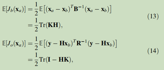
where H is a linearized observation operator. Based on Eqs 13 and 14 it is possible to iteratively correct the magnitudes of B and R, following

using the two indicators

where q is the current iteration.
Acting as scaling coefficients, the sequences {s <sub>b,q </sub>} and {s <sub>o,q </sub>} modify the error variance magnitude in the iterative process. It is worth reminding that both the analyzed state x <sub>a </sub> and the gain matrix K <sub>q </sub> are obtained using B <sub>q </sub> , R <sub>q </sub> which depend on s <sub>b,q </sub> and s <sub>o,q </sub>. When the correlation patterns of both B and R are well known, DI01 is equivalent to a maximum-likelihood parameter tuning, as pointed out in [28, 47].
Unlike other posterior covariance diagnosis/computations, such as [24, 26], the estimation of the full matrices is not needed in DI01. Instead, only the estimation of two scalar values (J <sub>b </sub>, J <sub>o </sub>) is required, which significantly reduce the computational cost. As a consequence, this method could be more appropriate for online covariance tuning.
Q: ↑ DI01为什么不需要对整个矩阵进行估计?因为增益是验证指标吗?
5.2 Desroziers iterative method (D05) in the observation space
The Desroziers diagnosis (D05)[24], subject to prior and posterior state-observation residuals has been widely applied in engineering problems, including numerical weather prediction[28] and hydrology [3]. The work of [24] proved that when B and R are well known a priori, the expectation of the analysis state should satisfy:

The difference between the left side and the right side of Eq 18,

↑ D05迭代方法的收敛指标,当收敛时,趋近0
can be used as a validation indicator of the R matrix estimation where ||.||<sub>F </sub> denotes the Frobenius norm. Applying this method, time variant observation/background data can contribute to the estimation of the R matrix because the expectation in Eq 18 could be evaluated using residuals at different time steps. When the B matrix is well known, an iterative process has been introduced to estimate the R matrix:

↑ D05迭代方法要求 B 矩阵已知~
based on the fixed-point theory [29]. The current analysis state x <sub>a,q </sub> is obtained using the specification of R <sub>q </sub> while x <sub>b </sub> , B, y remains invariant. As proved in [28, 29], under the assumption of sufficient observation data and well known B matrix, the iterative process of Eq 20 converges to the exact observation error covariance. However, as shown in [29], the intermediate matrices R <sub>q </sub> could be non-symmetric and possibly contain negative or complex eigenvalues, which is cumbersome for DA algorithms to deal with.
In practice, a posterior regularization at each iteration step is often required to ensure the positive definiteness of R <sub>q </sub> [29] where the first step of the regularization could be symmetrizing the estimated R <sub>q </sub> matrix, i.e.,

The spectrum of R <sub>q </sub> now contains only real numbers but they are not necessarily positive. The hybrid method[2] is a standard approach in ensemble-based DA methods to ensure the positive definiteness, which consists of combining a prior defined covariance matrix C with the one obtained from empirical estimation. We thus obtain the formulation of the regularized observation matrix R <sub>r,n </sub> :

↑ 正则化,为了满足正定性(实数)+非负性,
following Eq 21 with μ∈(0,1). The matrix C is often set as a diagonal matrix since it helps to enhance the matrix conditioning. In this work, we choose to set

↓ 正则化的观测矩阵收敛性仍未解决~
so that Tr(R <sub>q </sub>) will not be modified due to the post regularization. As mentioned in the discussion of [3, 29], the convergence of regularized observation matrices remains an open question. Therefore, a small iteration number is often assigned for D05 tuning in industrial problems (e.g., q = 2 in [3, 49]). Since the right side of Eq 20 can be estimated using residual quantities at different time steps, D05 is often used to deal with time series observation data (e.g., [3, 49]) when assuming the R matrix is time-invariant.
6 LSTM for error covariance estimation
6.1 Introduction of RNN and LSTM
LSTM, first introduced in [50], is a kind of RNN [31], capable of solving long-term dependency problems [51] that traditional RNN could not handle. As with other recurrent neural networks, LSTM has a chain-like structure. This structure is created by repeating the same module shown on the left side in Fig. 1. In addition, the repeating module comprises four neural networks instead of only one. The specific structure of the repeating module is on the right side in Fig. 1.
↑ 李宏毅老师的视频对RNN,讲的很详细~
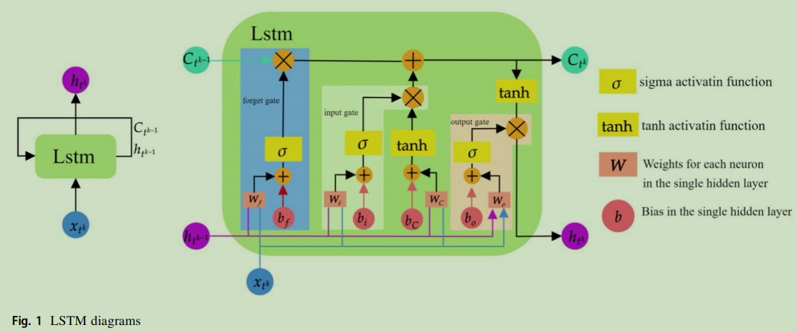
An essential part of LSTM is the cell state C <sub>t <sup>k-1 </sup> </sub> which is the long-term memory storing information about past behaviors. LSTM uses three gates with each composed out of a sigmoid layer neural network (single layer neural network with sigmoid activation function at the output layer) and a pointwise multiplication operation, to protect and control information of the cell state as shown in Fig. 1.
The first gate is the forget gate following:

where the recurrent variable h <sub>t <sup>k-1 </sup> </sub> summarizing all the information about past behaviors, x <sub>t <sup>k </sup> </sub> resuming information about current behaviors, and W <sub>f </sub> and b <sub>f </sub> are weights and bias, respectively, parameterizing the sigma layer neural network. The forget gate decides what kind of information is going to be ignored in C <sub>t <sup>k-1 </sup></sub>.
The second gate is the input gate, and it determines which new information is added into C <sub>t <sup>k-1 </sup> </sub> . This new information, $\tilde{\mathbf{C}}_{t^{k}}$, as conforming to

is attained by passing h <sub>t <sup>k-1 </sup> </sub> and x <sub>t <sup>k </sup> </sub> to a tanh layer neural network (single layer neural network with tanh activation function at the output layer) with parameters W <sub>c </sub> and b <sub>c </sub> .
$\tilde{\mathbf{C}}_{t^{k}}$ is then multiplied by weight coefficients i <sub>t <sup>k </sup> </sub> which is acquired by the input gate, i.e.,

i <sub>t <sup>k </sup> </sub> is applied to decide which new information would be employed to update C <sub>t <sup>k-1 </sup> </sub>.
Hence, the state cell C <sub>t <sup>k </sup> </sub> at the current time step t <sup>k </sup> can be attained using

Finally, the acquisition of h <sub>t <sup>k </sup> </sub> requires the participation of the output gate and a tanh activation function: first, the tanh activation function tanh is used to create a cell state candidate information tanh(C <sub>t <sup>k </sup> </sub>). tanh(C <sub>t <sup>k </sup> </sub>) is then multiplied by some weight coefficients following

to decide which information of tanh(C <sub>t <sup>k </sup> </sub>) would contribute to the obtainment of h <sub>t <sup>k </sup> </sub> . Among them, o <sub>t <sup>k </sup> </sub>, is generated by the output gate with neural network parameters W <sub>o </sub> and b <sub>o </sub> , i.e.,

6.2 LSTM for R matrix estimation using time series observation data (Q)
The tuning methods presented in Section 5 have been applied in various engineering applications with significant improvement of covariance specification and DA accuracy. However, these methods which require several applications of DA algorithms can be computationally expensive for high-dimensional problems. Another important drawback stands for the requirement of precise knowledge on either the correlation patterns of B and R (for DI01) or the full B matrix (for D05).
Q: ↑ 还是不能理解 DI01 做什么?correlation pattern 是 full matrix吗?
In this study, we aim to build a data-driven surrogate model for efficient online R matrix specification using LSTM. Unlike DI01 or D05, no specific knowledge about the error covariances or the state/observation dynamical systems other than the transformation operator H and the forward model M <sub>t <sup>k </sup>→t <sup>k+1 </sup></sub> (which is also indispensable for standard DA algorithms including variational methods and Kalman-filters) is required.
↑ 指出了本算法的需要,观测算子、前向模型,不需要,B和R的相关特定信息
😎~win+. emoji表情包
Algorithm 1:Simulated observations generating process

our main idea is to build a training set for the specific problem, including predefined time-invariant observation matrices {$\mathbf{R}^{[\text{iter}]}$} within certain range and generated dynamical observation vector {$\mathbf{y}_{t^{k}}^{[\text {iter }]}$}.
↑ 算法1:目的
Setting the dynamical observations {$\mathbf{y}_{t^{k}}^{[\text {iter }]}$} as the system input and the R matrices as output, LSTM networks are used to learn the error distribution across the underlying observation dynamics.
↑ 算法1:和LSTM的联系,LSTM的输入,输出,LSTM作用
More precisely, a real function $g^{\mathbf{R}}(.): \Phi_{\mathbf{R}} \longrightarrow \mathbb{R}^{m \times m}$ is predefined where $\Phi_{\mathbf{R}}$ is an empirically estimated real space which defines the range of a set of parameters, such as marginal error variance, correlation scale length [18] for computing the R matrices. The generated observation matrices {$\mathbf{R}^{[\text{iter}]}$} are set to be symmetric positive definite (SPD) thanks to the function $g^{\mathbf{R}}(.)$. Both $g^{\mathbf{R}}(.)$ and $\Phi_{\mathbf{R}}$ vary for different applications.
↑ 算法1:介绍了$\Phi_{\mathbf{R}}$,生成的R是对称正定的
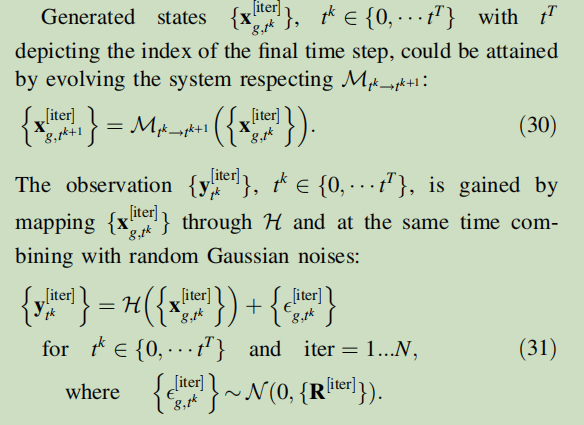
↑ 算法1:核心求解公式
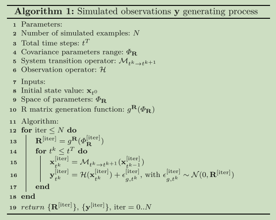
↑ 算法1:完整的观测模拟生成过程;
Algorithm 2: LSTM training and validation process
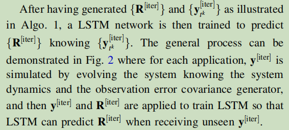


Different from classical covariance tuning algo-rithms, the LSTM network only makes use of historical observation data, requiring neither the background states nor the error covariance matrix. The advantage of using LSTM is more salient when the observation dimension is large, for example, millions or even billions, while such dimension is not uncommon in real-world applications [2, 7].
To estimate R, LSTM is first trained to learn: related variables
- – either which can be used to constitute the symmetry observation error covariance matrix (i.e., input variables of the g
<sup>R</sup>(.) function) in a parametric modeling; - –or elements of the R matrix (e.g., variables in the upper triangle and those in the diagonal of the covariance matrix) in a non-parametric modeling.
The whole process for R estimation using LSTM is described in Algorithm 2.
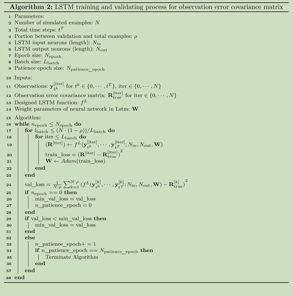
In Algorithm 2, it is suggested that LSTM training process is consisted of training and validation processes:
- the training process is comprised of the forward prediction and the backward neural network weight parameters updating processes;
- and validation process is used to predict desirable outputs or objectives and then calculate validation loss between predicted output and prior true output values.
- N_epoch indicates the number of times that the entire example data set is passed forward and backward through the LSTM during the training process.
- Early stopping, which terminates the training process when the validation loss reaches the minimum and is always the minimum value after N_patience_epoch epochs, is applied to reduce the LSTM training time.
It is important to note that the offline data generation and LSTM training processes need to be carried out individually for different DA applications (Fig 4).

7 Lorenz twin experiment
7.1 Twin experiment principle
In order to overcome the drawback that, in a realistic experiment, x <sub>true </sub> is usually unknown and y is often mixed with noises, twin experiment, in which a prototypical test case is selected to simulate real situations, is applied so as to provide x <sub>true </sub> for comparison.
↑ 解释了什么是孪生实验
In this experiment, a mapping is applied to some sampling true trajectory x <sub>true,t <sup>k </sup> </sub> at some points in space and time and arbitrary random noises are added to obtain simulated raw measurements y <sub>t <sup>k </sup> </sub> . DA is then implemented starting from the initial background state x <sub>b,t <sup>0 </sup> </sub> representing the prior information that could be obtained about corresponding state x <sub>true,t <sup>0 </sup> </sub> , along with initial raw measurement y <sub>t <sup>0 </sup> </sub> . The output state is then compared against x <sub>true </sub> , verifying the distance of these two states and minimizing it to evaluate and improve the performance of DA.
In this section, we use a twin experiment to evaluate the performance of applying DA to a simple Lorenz system in which raw measurement error covariance is estimated/adjusted using, respectively, DI01, D05 and LSTM.
7.2 Experiment set up (Q)
The Lorenz system, first studied by Edward Lorenz, is a system of ordinary differential equations. For certain parameter values and initial conditions, the Lorenz system is notable for having chaotic solutions, in particular the Lorenz attractor, toward which a system tends to evolve. The Lorenz 96 system[52] has been widely used as a prototypical test case to compare the performance of DA algorithms[34, 35, 53].
↑ 洛伦兹系统广泛应用于DA中
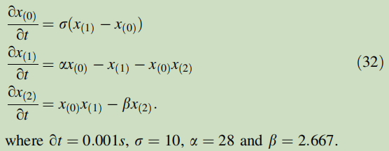
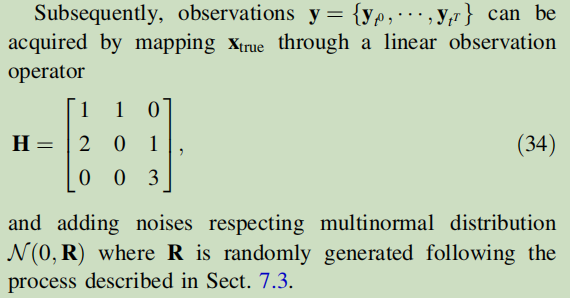
Here we build a twin experiment framework with a simple three dimensional Lorenz system in which the state vector is denoted as x=[x <sub>(0)</sub>, x <sub>(1)</sub>, x <sub>(2)</sub>]. The studied Lorenz system can be characterized as:
initial true state, initial background state →(Lorenz) true state, background
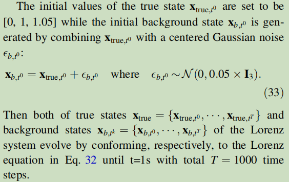
observations ← observation operator, noise
EnDA is then applied in this twin experiment to update the background ensemble using available observations.
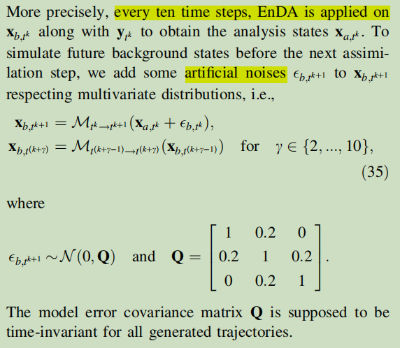
Q:↑ 同化窗口是 10 个时间步吗?
7.3 DA with LSTM-based covariance estimation
R matrix generation
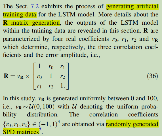
↑ 参数化R生成对称正定矩阵的网站:https://scikit-learn.org/stable/modules/generated/sklearn.datasets.make_spd_matrix.html
the input, output and structure of LSTM function
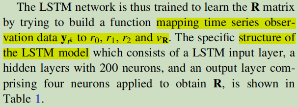

LSTM1000 and LSTM200:
↑ In this Lorenz twin experiment, two LSTM networks, respectively named as LSTM1000 and LSTM200 are designed with different input sizes of times series data. LSTM1000 is trained on a total of 1000 time steps for predicting the R matrix while LSTM200 makes use of only the first 200 time steps to simulate a realistic application where the time-invariant R matrix is estimated using historical data for improving future DA performance. The evaluation of both LSTM1000 and LSTM200, in terms of DA accuracy, is made using the full test dataset with 1000 times steps. By leveraging the LSTM model along with available observations, we can still perform DA algorithms even though R is not explicitly given. The results are then compared with the ones obtained using the exact R matrix.
7.4 Results
Prediction results of the non-parametric error covariance and the true values:
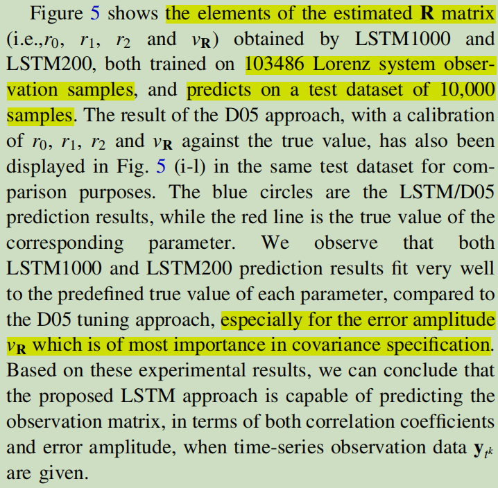

The averaged DA performance
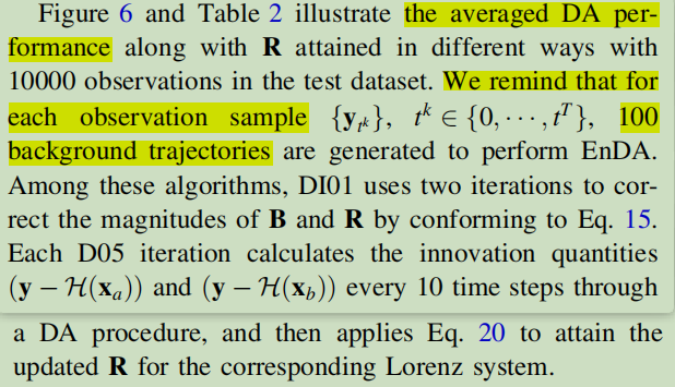
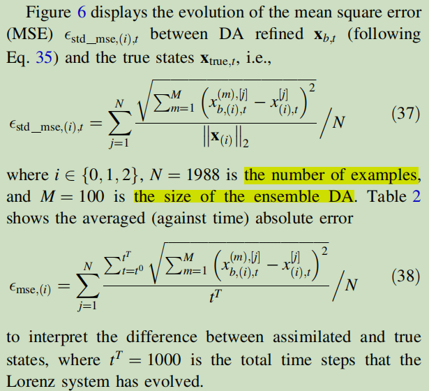


↑
averaged是因为EnDA有100个背景轨迹;
8 Application to shallow water equations
8.1 Experiment setup
For further evaluating the performance of error covariance estimation using LSTM when incorporated with predefined correlation kernels, we also set up a twin experiment framework with a simplified 2D shallow-water dynamical model, which is frequently used for testing data assimilation algorithms ( e.g., [26, 42]).
A cylinder of water is positioned in the middle of the study field with size 20mm × 20mm and released at the initial time step t <sup>k </sup>=t <sup>0 </sup> s (i.e., with no initial speed), leading to a non-linear wave-propagation. The dynamics of the water level h (in mm), as well as the horizontal and vertical velocity field (respectively denoted as u and v in 0.1m/s), is given by the nonconservative shallow water equations,
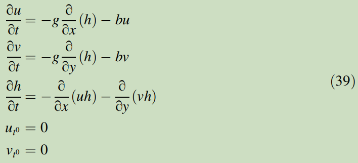
↑ 潜水模型
The evolution of the reference state (x <sub>true </sub>), together with the error-free model equivalent observations (i.e., H(x <sub>true </sub>)), is illustrated in Fig 8.
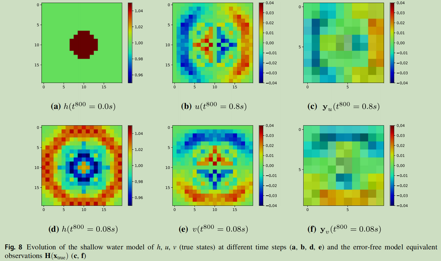
Spatially correlated prior observation errors are generated artificially and combined with the transformation operator to simulate real-time observations. More precisely, the observations are generated from the model equivalent H(x <sub>true </sub>) separately for the fields u and v. H is defined as a sparse matrix to imply the fact that measurements in real-world applications are sparser than true states due to the interference existing in the former situations as well as the limited performances of sensors.
↑ 这里对H算子与观测的关系说的非常到位,对H算子的稀疏性也讲的很好
As shown in Fig 7, the spatial observations at time t <sup>k </sup> is defined as the average of u <sub>t <sup>k </sup> </sub> and v <sub>t <sup>k </sup> </sub> in a 2 × 2 cells area with an observation error ε <sub>y <sub>t <sup>k </sup> </sub></sub> ,

and identical for y <sub>v,i,j,t <sup>k </sup> </sub> .
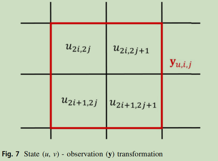
Therefore, the dimension of the observation vector y = [ y <sub>u,t <sup>k </sup> </sub>, y <sub>v,t <sup>k </sup> </sub>] is 200.
↑ 上面介绍的是某一时刻的观测是什么,H 观测算子依此构建
In this experiment, we suppose that the observation error ε <sub>y <sub>u,i,j,t <sup>k </sup> </sub></sub> and ε <sub>y <sub>v,i,j,t <sup>k </sup> </sub></sub> , respectively of the velocity fields u and v, follow the same Gaussian distribution N(0,R). Thus, the observation error covariance in this shallow water system can be fully characterized by a 100 × 100 R matrix after the observations (originally in a 2D grid) being converted to a 1D vector.
↑ 上面介绍的是某一时刻观测误差协方差的维数
Here we adopt a different parameterization of the R matrix thanks to an isotropic correlation function ψ <sub>R </sub>(.),

where D=[D
<sub>0</sub>,…, D<sub>99</sub>], representing the error variances in the 2D (10 × 10) velocity field. Each element of D is generated individually following an uniform distribution,
which produces only positive elements to guarantee the positive definiteness of R.
ψ
<sub>R</sub>(.) is the second-order auto-aggressive (also known as Balgovind) function,
where L
<sub>R</sub>is the correlation scale length, fixed as L<sub>R</sub>= 10 in this application. r denotes the correlation scale length in the 2D space and is also generated uniformly with r ~U(1,5).Being part of Matern kernels, the SOAR function is often used in DA for prior error covariance modeling [6, 26] thanks to its smoothness and good conditioning.
↑ 上面介绍了观测误差协方差的构建
The simulation of x <sub>b,t <sup>k </sup> </sub>=[u <sub>b,t <sup>k </sup> </sub>, v <sub>b,t <sup>k </sup> </sub>] via the same discretization of Eq 39 (except the initial conditions) is used as background states at time t <sup>k </sup> in the DA modeling. Similar to the Lorenz experiment(i.e., Eq 35), {x <sub>b,t <sup>k </sup> </sub>} is acquired by combining {x <sub>a,t <sup>k </sup> </sub>} with randomly generated Gaussian errors, while {x <sub>a,t <sup>k </sup> </sub>} is obtained every 100 time steps (i.e., 0.01s) from ensemble DA with time series observation data {y <sub>t <sup>k </sup> </sub>} and the estimated observation error covariance R.
↑ 上面介绍了某一时刻的背景场是什么
8.2 DA with LSTM estimated R
As with the Lorenz experiment, simulated observations {y <sub>t <sup>k </sup> </sub>}, generated in the same process with that in the Lorenz system, are used as input training data for the LSTM model, while the D vector and the correlation scale r served as training output.
↑ 上面介绍了浅水试验LSTM模型训练集的输入和输出
The specific structure of this LSTM network is shown in Table 3. This model has the same structure as the one of the Lorenz systems shown in Table 1, except the input and output dimensions. Besides, two types of LSTM are also proposed as what have been realized in the Lorenz system: LSTM1000 employs the whole 1000 time steps observation data as LSTM training and prediction inputs while LSTM200 makes use of only the first 200 time steps of observation data as the LSTM inputs.

↑ 上面介绍了浅水试验LSTM模型结构,两个试验
After the LSTM is well trained on the training set of 173000 generated observation trajectories in this experiment, R can be gained even only observation time-series data {y <sub>t <sup>k </sup> </sub>} is acknowledged.
↑ ...
Similar to the Lorenz system, EnDA is performed here with an ensemble of 100 state trajectories initialized from the same initial state x <sub>t <sup>0 </sup> </sub> for each observation series. EnDA takes place every 200 time steps with the R matrix estimated through different methods.
↑ EnDA 集合,EnDA 同化窗口
8.3 Results
Pycharm 实现 code
Git托管(待)
目前保存在D盘;
界面MATLAB化+环境配置
为了使得pycharm更像MATLAB,:
主题设置为 白色;
勾选
Run with Python Console,在运行完文件后,能在Python Console看到变量;
右键执行所选代码,能在Python Console看到变量;
pycharm不会将当前文件目录自动加入自己的sourse_path。右键make_directory as–>sources path将当前工作的文件夹加入source_path就可以了。这样可以在同目录下import其它py文件。
文件夹加入source_path后会显示成蓝色。
其实pycharm很强大的~~以前是自己了解的不够多~
有些MATLAB那味道了~~

怎么感觉pycharm比matlab还好用呀~~😊
在pycharm上以项目的形式打开
LSTM_Covariance-main文件夹,通过Anaconda,为项目创建一个新环境
为环境安装相关python包(库)
numpy
scipy
matplotlib
keras
tensorflow
sklearn
pandas
进入 Anaconda Prompt,输入:
conda info -e
conda activate LSTM_Covariance-main
pip install tensorflow
参考资料
pycharm新建项目环境设置详解:https://blog.csdn.net/weixin_38858443/article/details/108966449
- 项目、解释器、环境几个概念的理解
- 在pycharm为项目新建一个新环境
Pycharm中运行Python代码的几种方式:https://blog.csdn.net/JHON07/article/details/78966837
- 右键,run,ok~~
PyCharm配置anaconda环境 安装第三方库:https://blog.51cto.com/u_15284226/2992785
Pycharm在运行过程中,**查看每个变量的操作(show variables)**:http://www.deiniu.com/article/188284.htm
- 让你的Pycharm用得和matlab一模一样!:https://zhuanlan.zhihu.com/p/337278800?ivk_sa=1024320u
为什么用pycharm在同目录下import,pycharm会报错,但是实际可以运行?:
Lorenz
simulated_data_generation.py (QT)
simulated_data_generation.py released in 2022-02-26
整个运行时间
运行开始时间:17:55
运行结束时间:20:50
.ravel 矩阵向量化.concatenate axis=0 数组拼接y = np.dot(H,x) #why this is this expression to calculate y?这个 x ,在论文7.2中指出是x
<sub>true</sub>,而代码中的 x 根据7.2中公式(33)应该是x
<sub>b</sub>,QT:矛盾了吗?
猜测:我觉得应该是代码出了问题
代码中出现了两次 x
<sub>true</sub>的定义,有一个应该是x<sub>b</sub>;从同化公式可以看出,y应该等于H(x
<sub>true</sub>) ,如果观测数据y等于H(x<sub>b</sub>),那还需要同化什么呀,直接x<sub>a</sub>=x<sub>b</sub>。可以看看后面作者是怎么同化的~
往下看~
整个py的作用,6中的算法1,7.2部分,生成训练集;
simulated_data_generation.pyreleased in 2022-02-26 最开始的代码
# -*- coding: utf-8 -*-
# generate the trainning set for keras regression

import numpy as np
from scipy.optimize import fmin
from scipy.optimize import fmin_l_bfgs_b

#from scipy.optimize import fmin_ncg
from scipy.linalg import sqrtm
import math


from constructB import *
from lorentz_attractor import *

import matplotlib.pyplot as plt

import matplotlib.gridspec as gridspec
import time
import random
import lorentz_attractor
import sklearn
from sklearn import datasets

import os

if not os.path.isdir('lorenz_cov_train_v2'):
    os.makedirs('lorenz_cov_train_v2')

#######################################################################

def correlation_from_covariance(covariance):
    v = np.sqrt(np.diag(covariance))
    outer_v = np.outer(v, v)
    correlation = covariance / outer_v   #https://www.mygreatlearning.com/blog/covariance-vs-correlation/
    correlation[covariance == 0] = 0
    return correlation

######################################################################
#define matrix R by extra-diagonal elements
def R_covariance_dim3(r1,r2,r3):
    M = np.zeros((3,3))
    M[0,1] = r1
    M[0,2] = r2
    M[1,2] = r3
    M = M + M.T
    M += np.eye(3)
    return M

################################################################################
#######################################################################
def cov_to_cor(M): # from a covariance matrix to its associated correlation matrix
    inv_diag_M=np.linalg.inv(sqrtm(np.diag(np.diag(M))))
    cor_M = np.dot(inv_diag_M, np.dot(M,inv_diag_M))
    return cor_M


def lorenz_1step(x, y, z, s=10, r=28, b=2.667,dt = 0.001):
    x_dot, y_dot, z_dot = lorenz(x, y, z)
    x_next = x + (x_dot * dt)
    y_next = y + (y_dot * dt)
    z_next = z + (z_dot * dt)
    return x_next, y_next, z_next

def VAR_3D(xb,Y,H,B,R): #booleen=1 garde la trace
    xb1=np.copy(xb)
    xb1.shape=(xb1.size,1)
    Y.shape = (Y.size,1)
    dim_x = xb1.size
    K=np.dot(B,np.dot(np.transpose(H),np.linalg.inv(np.dot(H,np.dot(B,np.transpose(H)))+R))) #matrice de gain, Kalman gain
    A=np.dot(np.dot((np.eye(dim_x)-np.dot(K,H)),B),np.transpose((np.eye(dim_x)-np.dot(K,H))))+np.dot(np.dot(K,R),np.transpose(K))  #not the kalman filter expression???
    vect=np.dot(H,xb1)
    xa=np.copy(xb1+np.dot(K,(Y-vect)))

    return xa,A   #xa is the new estimated data, A is the new covariance,
###################################################################################

###################################################################################
    #parameters
num_steps = 1000
H = np.array([[1,1,0],[2,0,1],[0,0,3]])
R = 0.001*np.array([[1,0.4,0.1],[0.4,1,0.4],[0.1,0.4,1]])

B =0.01*np.array([[1,0.2,0.],[0.2,1,0.2],[0.,0.2,1]])
#Q = 0.0001*np.eye(3)

###################################################################################
#save the trainning set for different R
trainning_set = np.zeros((1,num_steps*3+3+4))

###################################################################################

#############################################################################
    # true states vector 3 * number_steps
xs,ys,zs = lorenz_attractor(s=10, r=28, b=2.667, dt = 0.001, num_steps=1000)

x_true = np.zeros((3,num_steps+1))

x_true[0,:] = np.copy(xs)
x_true[1,:] = np.copy(ys)
x_true[2,:] = np.copy(zs)


###############################################################################
for ii in range(2000):
    if ii%100 ==0:
        print(ii)

# construct observations

#=========================================================================
    #generate x with noise
    for repetation in range(10):
        xs,ys,zs = lorenz_attractor(s=10, r=28, b=2.667, dt = 0.001, num_steps = 1000,x0 = 0.+np.random.normal(0, 0.05),
                                    y0=1.+np.random.normal(0, 0.05),z0=1.05+np.random.normal(0, 0.05))

        x_true = np.zeros((3,num_steps+1))

        x_true[0,:] = np.copy(xs)
        x_true[1,:] = np.copy(ys)
        x_true[2,:] = np.copy(zs)

#=========================================================================

        y_true = np.zeros((3,num_steps+1))
        y_obs = np.zeros((3,num_steps+1))

        v = np.random.uniform(0,100.)
        R = correlation_from_covariance(sklearn.datasets.make_spd_matrix(3))  #SPD covariance

        r1 = R[0,1]
        r2 = R[0,2]
        r3 = R[1,2]

        R = v*R
        for i in range(num_steps+1):
            print("sample time: ",ii)
            print("iteration time: ",i)
            x = x_true[:,i]
            x.shape = (x.size,1)
            y = np.dot(H,x)               #why this is this expression to calculate y?
            y.shape = (y.size,)
            y_true[:,i] = y

            y_noise = np.random.multivariate_normal(np.zeros(3),R)
            y_noise.shape = (y_noise.size,)
            y_noise += y
            y_obs[:,i] = y_noise

            parameters = np.array([r1,r2,r3,v]) #output for deep learning regression
                        #train_row = np.concatenate((y_obs.ravel(),x_true.ravel())) #input for deep learning    #what are the functionalities of these r ->covaraicen! why v is not necessary???
            train_row = y_obs.ravel()
            train_row = np.concatenate((train_row.ravel(),parameters))

        train_row.shape = (1,train_row.size)
        trainning_set = np.concatenate((trainning_set,train_row), axis=0)

        # if repetation+ii*10==5000:

        #     np.savetxt(f"lorenz_cov_train_v2/trainset_withx_steps1000_test_{10000+repetation+ii*10}.csv", trainning_set, delimiter=",")

trainning_set = trainning_set[1:,:]
#####################################################################################""
np.savetxt("lorenz_cov_train_v2/trainset_withx_steps1000_test8.csv", trainning_set, delimiter=",")
simulated_data_generation.py 在released in 2022-02-26 基础上,进行注释
# -*- coding: utf-8 -*-
# generate the trainning set for keras regression

import numpy as np
from scipy.optimize import fmin
from scipy.optimize import fmin_l_bfgs_b

#from scipy.optimize import fmin_ncg
from scipy.linalg import sqrtm
import math


from constructB import *
from lorentz_attractor import *

import matplotlib.pyplot as plt

import matplotlib.gridspec as gridspec
import time
import random
import lorentz_attractor
import sklearn
from sklearn import datasets

import os

if not os.path.isdir('lorenz_cov_train_v2'):
    os.makedirs('lorenz_cov_train_v2')

#######################################################################

def correlation_from_covariance(covariance):
    '''
    Given:
        covariance: 对称正定矩阵
    Returns:
        correlation: (-1,1) 的对称正定矩阵,相关系数

    '''
    v = np.sqrt(np.diag(covariance))
    outer_v = np.outer(v, v)
    correlation = covariance / outer_v   #https://www.mygreatlearning.com/blog/covariance-vs-correlation/
    correlation[covariance == 0] = 0
    return correlation

######################################################################
#define matrix R by extra-diagonal elements
def R_covariance_dim3(r1,r2,r3):
    M = np.zeros((3,3))
    M[0,1] = r1
    M[0,2] = r2
    M[1,2] = r3
    M = M + M.T
    M += np.eye(3)
    return M

################################################################################
#######################################################################
def cov_to_cor(M): # from a covariance matrix to its associated correlation matrix
    inv_diag_M=np.linalg.inv(sqrtm(np.diag(np.diag(M))))
    cor_M = np.dot(inv_diag_M, np.dot(M,inv_diag_M))
    return cor_M


def lorenz_1step(x, y, z, s=10, r=28, b=2.667,dt = 0.001):
    x_dot, y_dot, z_dot = lorenz(x, y, z)
    x_next = x + (x_dot * dt)
    y_next = y + (y_dot * dt)
    z_next = z + (z_dot * dt)
    return x_next, y_next, z_next

def VAR_3D(xb,Y,H,B,R): #booleen=1 garde la trace
    xb1=np.copy(xb)
    xb1.shape=(xb1.size,1)
    Y.shape = (Y.size,1)
    dim_x = xb1.size
    K=np.dot(B,np.dot(np.transpose(H),np.linalg.inv(np.dot(H,np.dot(B,np.transpose(H)))+R))) #matrice de gain, Kalman gain
    A=np.dot(np.dot((np.eye(dim_x)-np.dot(K,H)),B),np.transpose((np.eye(dim_x)-np.dot(K,H))))+np.dot(np.dot(K,R),np.transpose(K))  #not the kalman filter expression???
    vect=np.dot(H,xb1)
    xa=np.copy(xb1+np.dot(K,(Y-vect)))

    return xa,A   #xa is the new estimated data, A is the new covariance,
###################################################################################

###################################################################################
#parameters
num_steps = 1000
H = np.array([[1,1,0],[2,0,1],[0,0,3]])
R = 0.001*np.array([[1,0.4,0.1],[0.4,1,0.4],[0.1,0.4,1]])

B =0.01*np.array([[1,0.2,0.],[0.2,1,0.2],[0.,0.2,1]])
#Q = 0.0001*np.eye(3)

###################################################################################
#save the trainning set for different R
trainning_set = np.zeros((1,num_steps*3+3+4))
    #加3的原因:Lorenz 系统每个参数的时间节点个数,比步长数多 1,有3个参数,加3
    #加4的原因:R 矩阵生成的4个参数

###################################################################################

#############################################################################
# true states vector 3 * number_steps
xs,ys,zs = lorenz_attractor(s=10, r=28, b=2.667, dt = 0.001, num_steps=1000)

x_true = np.zeros((3,num_steps+1)) # 真实场

x_true[0,:] = np.copy(xs)
x_true[1,:] = np.copy(ys)
x_true[2,:] = np.copy(zs)


###############################################################################
for ii in range(2000):  # ii = 0   算法1  中的iter?
    if ii%100 ==0:
        print(ii)

# construct observations

#=========================================================================
    for repetation in range(10):  # repetation = 0
        # 背景场 的生成
        xs,ys,zs = lorenz_attractor(s=10, r=28, b=2.667, dt = 0.001, num_steps = 1000,x0 = 0.+np.random.normal(0, 0.05),
                                    y0=1.+np.random.normal(0, 0.05),z0=1.05+np.random.normal(0, 0.05))

        x_true = np.zeros((3,num_steps+1)) # 背景场,这里只对初始值进行噪声干扰,是因为lorenz是个混沌系统;

        x_true[0,:] = np.copy(xs)
        x_true[1,:] = np.copy(ys)
        x_true[2,:] = np.copy(zs)

#=========================================================================

        y_true = np.zeros((3,num_steps+1)) #
        y_obs = np.zeros((3,num_steps+1)) #

        # R 的构建
        v = np.random.uniform(0,100.)
        R = correlation_from_covariance(sklearn.datasets.make_spd_matrix(3))  #SPD covariance

        r1 = R[0,1]
        r2 = R[0,2]
        r3 = R[1,2]

        R = v*R

        # 训练数据集 的构建:Lorenz 3 个参数的时间节点(3*1001),R 的 4 个参数 (+4)
        for i in range(num_steps+1): # i=0
            print("sample time: ",ii) #采样次数
            print("iteration time: ",i) #迭代次数
            # 观测 y 的生成
            x = x_true[:,i]
            x.shape = (x.size,1)
            y = np.dot(H,x)               #why this is this expression to calculate y?
            y.shape = (y.size,)
            y_true[:,i] = y

            y_noise = np.random.multivariate_normal(np.zeros(3),R)
            y_noise.shape = (y_noise.size,)
            y_noise += y
            y_obs[:,i] = y_noise

            # 拼接上 R 的 4 个参数
            parameters = np.array([r1,r2,r3,v]) #output for deep learning regression
                        #train_row = np.concatenate((y_obs.ravel(),x_true.ravel())) #input for deep learning    #what are the functionalities of these r ->covaraicen! why v is not necessary???
            train_row = y_obs.ravel()  # .ravel 矩阵向量化,x = np.array([[1,2],[3,4]]),则print(np.ravel(x)) = [1 2 3 4]
            train_row = np.concatenate((train_row.ravel(),parameters)) # .concatenate 数组拼接

        train_row.shape = (1,train_row.size) # .shape
        trainning_set = np.concatenate((trainning_set,train_row), axis=0) # .concatenate axis=0 数组拼接

        # if repetation+ii*10==5000:

        #     np.savetxt(f"lorenz_cov_train_v2/trainset_withx_steps1000_test_{10000+repetation+ii*10}.csv", trainning_set, delimiter=",")

trainning_set = trainning_set[1:,:] # 不要第一行,全是 0 的那一行;
#####################################################################################""
np.savetxt("lorenz_cov_train_v2/trainset_withx_steps1000_test8.csv", trainning_set, delimiter=",")
QT:为什么线性观测算子H是固定的那个矩阵?为什么H(x)加上个多元误差的协方差分布,就变成观测了?(因为DA中,观测也是有误差的?)
lorenz_lstm200.py
lorenz_lstm200.py released in 2022-02-26
报错:
ImportError: cannot import name 'Adam' from 'keras.optimizers' (D:\Program Files (x86)\Anaconda3\envs\LSTM_Covariance-main\lib\site-packages\keras\optimizers.py)from tensorflow.keras.optimizers import Adam整个运行时间
运行开始时间:11:40
运行结束时间:14:20
相关代码知识点
# 相对路径解决办法 #train_data = data_set_order('D:/LSTM_Covariance-main/lorenz/lorenz_cov_train_v2/trainset_withx_steps1000_test8.csv') #os.getcwd() os.chdir('D:/LSTM_Covariance-main/lorenz/') # -2表示的意思 train_data = np.array(pd.read_csv(file))[:-2,:] #取这个数组从第一行到倒数第三行,最后两行被丢弃了。 # .insert axis=1 列插入 train_data=np.insert(r0,[i+1 for i in range(r0.shape[1])],r1,axis=1) #.concateenate axis=1 列合并` train_data=np.concatenate((train_data,r3),axis=1) # .random.shuffle 打乱行的顺序 np.random.shuffle(train_data ) # 与matlab不一样的一点:索引 input_data = train_data[:,0:603] output_data = train_data[:,603:] #出现两次 603 ,索引的数据重复了吗?没有 # 可以对中文变量进行赋值,意义在于,可以在pycharm看到变量的大纲 P03_LSTM模型结构和运行 = 0 # pycharm中plt.show()不显示图像解决办法 import matplotlib import matplotlib.pyplot as plt matplotlib.use('TKAgg')#加上这行代码即可,agg是一个没有图形显示界面的终端,常用的有图形界面显示的终端有TkAgg等lorenz_lstm200.pyreleased in 2022-02-26 最开始的代码
# -*- coding: utf-8 -*-
"""
Created on Wed Jan  6 13:39:58 2021

@author: siboc
"""

import numpy as np
import scipy
import math
import matplotlib.pyplot as plt


from keras.models import Sequential
from keras.layers import Dense
from sklearn.metrics import r2_score
import tensorflow as tf
import keras.backend as K
# check scikit-learn version

# check scikit-learn version
import sklearn
from sklearn.linear_model import LinearRegression
from sklearn.datasets import make_regression
from sklearn.neighbors import KNeighborsRegressor
from sklearn.tree import DecisionTreeRegressor
import pandas as pd

def data_set_order(file):
	train_data = np.array(pd.read_csv(file))[:-2,:]
	r0=train_data[:,:1001][:,:201]
	r1=train_data[:,1001:2002][:,:201]
	r2=train_data[:,2002:3003][:,:201]
	r3=train_data[:,3003:]
	r3[:,-1]=r3[:,-1]/100
	train_data=np.insert(r0,[i+1 for i in range(r0.shape[1])],r1,axis=1)
	train_data=np.insert(train_data,[(i+1)*2 for i in range(int(train_data.shape[1]/2))],r2,axis=1)
	train_data=np.concatenate((train_data,r3),axis=1)
	return train_data

#input
train_data = data_set_order('lorenz_cov_train_v2/trainset_withx_steps1000_test8.csv')
print("train_data shape: ",train_data.shape)


# train_data1 = data_set_order('lorenz_cov_train/trainset_withx_repeat10bis3.csv')
# print("train_data1 shape: ",train_data1.shape)

# train_data2 = data_set_order('lorenz_cov_train/trainset_withx_repeat10bis4.csv')
# print("train_data2 shape: ",train_data2.shape)

# train_data3 = data_set_order('lorenz_cov_train/trainset_withx_repeat10bis5.csv')
# print("train_data3 shape: ",train_data3.shape)

# train_data4 = data_set_order('lorenz_cov_train/trainset_withx_repeat10bis6.csv')
# print("train_data4 shape: ",train_data4.shape)

# train_data5 = data_set_order('lorenz_cov_train/trainset_withx_repeat10bis7.csv')
# print("train_data5 shape: ",train_data5.shape)

# train_data6 = data_set_order('lorenz_cov_train/trainset_withx_repeat10bis8.csv')
# print("train_data6 shape: ",train_data6.shape)

#size: num_steps*3,r1,r2,r3,v


#########################################################################################

#train_data = np.array(pd.read_csv('data_1000steps/trainset_withx_1000steps.csv'))
#
#
#train_data1 = np.array(pd.read_csv('data_1000steps/trainset_withx_1000stepsbis1.csv'))
#
#train_data2 = np.array(pd.read_csv('data_1000steps/trainset_withx_1000stepsbis2.csv'))
#
#train_data3 = np.array(pd.read_csv('data_1000steps/trainset_withx_1000stepsbis3.csv'))


# train_data = np.concatenate((train_data6,train_data5),axis = 0)

# train_data = np.concatenate((train_data,train_data4),axis = 0)

# train_data = np.concatenate((train_data,train_data3),axis = 0)

# train_data = np.concatenate((train_data,train_data2),axis = 0)

# train_data = np.concatenate((train_data,train_data1),axis = 0)

# train_data = np.concatenate((train_data,train_data0),axis = 0)

# train_data=train_data[:120000,:]


#weightstrain_data[:,604:]
np.random.shuffle(train_data )

input_data = train_data[:,0:603]
output_data = train_data[:,603:]


########################################################################
train_part = 0.97

threshold = int(train_part*train_data.shape[0])


##########################################################################

train_input = input_data[:threshold]

print("input_data shape: ",input_data.shape)

train_output = output_data[:threshold]

print("output_data shape: ",output_data.shape)


test_input = input_data [threshold:]

true_test_output = output_data[threshold:]


X1 = train_input
Y1 = train_output

X2 = test_input
#Y2 = ValidationSet_Y

############################################################################


#def my_loss_fn(y_true, y_pred):
#
#    return K.mean(K.abs(y_true - y_pred) * weight)

# ========================================================================================
from keras.layers import LSTM,Dropout
from keras.layers import TimeDistributed
from keras.callbacks import EarlyStopping
from keras.callbacks import ModelCheckpoint
from keras.optimizers import Adam


# save data
import os
import json
import pickle

if not os.path.isdir('save_data_v2'):
	os.makedirs('save_data_v2')

hidden_size=200

input_sample=input_data.shape[0]  #for one sample


output_sample=output_data.shape[0]

input_data=input_data.reshape(input_sample,201,3)  #201 is the time steps in data_generation
output_data=output_data.reshape(output_sample,4)

use_dropout=True
model = Sequential()
model.add(LSTM(hidden_size,input_shape=(201,3)))

model.add(Dense(4))
# opt = Adam(lr=0.0001)
model.compile(loss='mean_squared_error', optimizer='Adam', metrics=['mae'])
print(model.summary())

es=EarlyStopping(monitor='val_loss',mode='min',verbose=1,patience=50)
# modelcheckpoint
mc=ModelCheckpoint('save_data_v2/sequentiallstm200_ing.h5',monitor='val_loss',mode='min',save_best_only=True,verbose=1)

history=model.fit(input_data, output_data, validation_split=0.1, epochs=100, batch_size=128, verbose=1,callbacks=[es,mc])


# model.save('save_data/sequentiallstm2')
model.save('save_data_v2/sequentiallstm200_ing_f.h5')

# https://stackoverflow.com/a/44674337/10349608
with open('save_data_v2/sequentiallstm200_ing_history.pickle', 'wb') as file_his:
	pickle.dump(history.history, file_his)


# Calculate predictions
PredTestSet = model.predict(X1.reshape(X1.shape[0],201,3))
PredValSet = model.predict(X2.reshape(X2.shape[0],201,3))


plt.plot(history.history['loss'])
plt.plot(history.history['val_loss'])
plt.title('Model loss')
plt.ylabel('Loss')
plt.xlabel('Epoch')
plt.legend(['Train', 'Test'], loc='upper left')
#plt.savefig('figure_dp/loss_trace.eps', format='eps',bbox_inches='tight')
plt.show()


plt.plot(PredValSet[:,2],true_test_output[:,2],'o', color='blue',markersize=5)
#plt.plot(list(range(0,1,0.1)),list(range(0,1,0.1)),'k')
plt.show()

plt.plot(PredValSet[:,3],true_test_output[:,3],'o',color='blue',markersize=5)
#plt.plot(list(range(0,1,0.1)),list(range(0,1,0.1)),'k')
plt.show()


# predint = model.predict(train_input[:3000])

# trueint = train_output[:3000]


# plt.plot(predint[:,3],trueint[:,3],'o', color='blue',markersize=5)
# #plt.plot(list(range(0,1,0.1)),list(range(0,1,0.1)),'k')
# plt.show()
QT:Tensorflow-keras与keras的区别
Tensorflow-keras与keras的区别:https://www.jianshu.com/p/135b2ee61a1c
如果你需要任何一个上述tf.keras的特有特性的话,那当然应该选择tf.keras。
如果后端可互换性对你很重要的话,那选择keras。
如果以上两条对你都不重要的话,那选用哪个都可以。
Shallow water:希望能对lorenz中遇到的问题,得到启发~
算法1,没给出同化的具体程序~~🤮
2022-02-28:LSTM_Covariance-main.zip
链接:https://pan.baidu.com/s/1Dtx-p4LRHhIGjTilVvgw-g
提取码:8egl
–来自百度网盘超级会员V5的分享


