<center>参考资料:nansencenter-DA-tutorials-2021 </center>
Git托管(待)
目前保存在D盘中
README.md:Introduction to data assimilation and the EnKF
Cloud computing
Jump right in using one of these cloud computing providers:
(requires Google login)
(no login but can be slow to start)
Overview
- Interactive (Jupyter notebook)
- Contains theory, code (Python), and exercises.
- Recommendation: work in pairs.
- Each tutorial takes ≈75 min.
- The tutor will circulate to assist with the exercises,
and summarize each section after you have worked on them.
Instructions for working locally
You can also run these notebooks on your own (Linux/Windows/Mac) computer. This is a bit snappier than running them online.
Prerequisite: Python 3.7.
If you’re an expert, setup a python environment however you like. Otherwise: Install Anaconda, then open the Anaconda terminal and run the following commands:conda create --yes --name my-env python=3.7 conda activate my-env python --versionEnsure the printed version is 3.7.
Keep using the same terminal for the commands below.Install:
- Download and unzip (or
git clone) this repository (see the green button up top) - Move the resulting folder wherever you like
cdinto the folder- Install requirements:
pip install -r path/to/requirements.txt
- Download and unzip (or
Launch the Jupyter notebooks:
- Launch the “notebook server” by executing:
jupyter-notebook
This will open up a page in your web browser that is a file navigator. - Enter the folder
DA-tutorials/notebooks, and click on a tutorial (T1... .ipynb).
- Launch the “notebook server” by executing:
Jupyter 实现 code
环境搭建+打开Jupyter
下载github项目的文件夹
DA-tutorials-master,在pycharm上以项目的形式打开DA-tutorials-master文件夹,通过Anaconda,为项目创建一个新环境DA-tutorials-master。(py3.7版本)在pycharm~~
安装依赖包
requirements.txt;pycharm下

pycharm上可能还是会出现一些包没有安装上
建议在Anaconda Prompt中下载(这种批量安装形式,太棒了~~)
conda info -e
conda activate DA-tutorials-master

进入下载的github项目的文件夹目录下
d:
cd D:\DA-tutorials-master

pip install -r requirements.txt
在Anaconda Prompt中激活
DA-tutorials-master环境,进入下载的github项目的文件夹目录下,jupyter-notebook在
jupyter验证是不是对应的环境: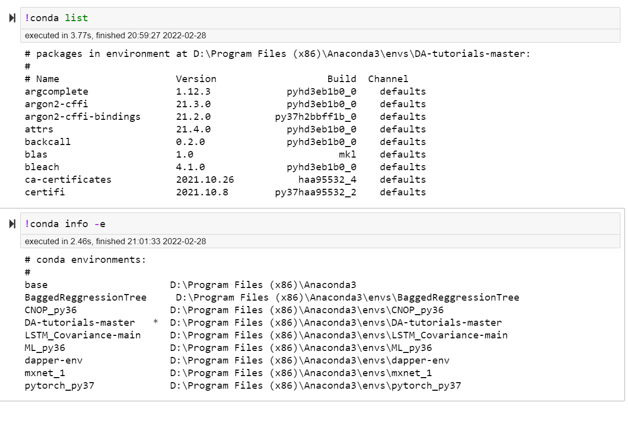
T1: Data assimilation (DA) & the ensemble Kalman filter (EnKF)

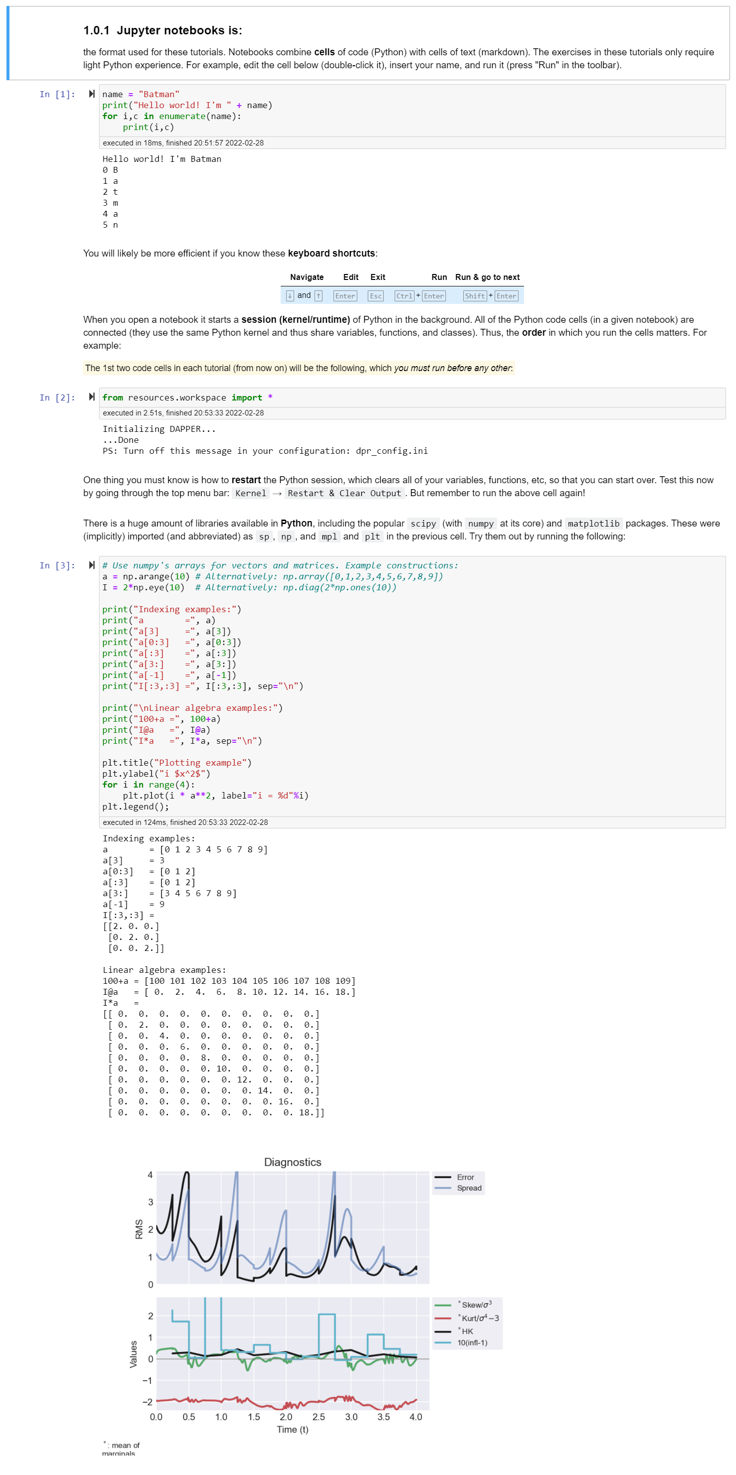
Jupyter notebooks is:
Data assimilation (DA) is:
- the calibration of big models with big data;
- the fusion of forecasts with observations.
This illustrated on the right (source: Data Assimilation Research Team, www.aics.riken.jp) as a “bridge” between data and models.
The problem of DA fits well within the math/stats theory of state estimation and sequential inference. A concise theoretical overview of DA is given by Wikle and Berliner: A Bayesian tutorial for data assimilation
Modern DA builds on state estimation techniques such as the Kalman filter (KF), which is an algorithm that recursively performs a form of least-squares regression. It was developed to steer the Apollo mission rockets to the moon, but also has applications outside of control systems, such as speech recognition, video tracking, and finance. An introduction by pictures is provided by Tim Babb. An interactive tutorial has been made by Roger Labbe.
When it was first proposed to apply the KF to DA (specifically, weather forecasting), the idea sounded ludicrous because of some severe technical challenges in DA (vs. “classic” state estimation):
- size of data and models;
- nonlinearity of models;
- sparsity and inhomogeneous-ness of data.
Some of these challenges may be recognized in the video below.
The EnKF is:
an ensemble (Monte-Carlo) formulation of the KF that manages (fairly well) to deal with the above challenges in DA.
For those familiar with the method of 4D-Var, further advantages of the EnKF include it being:
- Non-invasive: the models are treated as black boxes, and no explicit Jacobian is required.
- Bayesian:
- provides ensemble of possible realities;
- arguably the most practical form of “uncertainty quantification”;
- ideal way to initialize “ensemble forecasts”;
- uses “flow-dependent” background covariances in the analysis.
- provides ensemble of possible realities;
- Embarrassingly parallelizable:
- distributed across realizations for model forecasting;
- distributed across local domains for observation analysis.
The rest of this tutorial provides an EnKF-centric presentation of DA; it also has a theoretical companion.
DAPPER example
This tutorial builds on the underlying package, DAPPER, made for academic research in DA and its dissemination. For example, the code below is taken from DAPPER/example_1.py. It illustrates DA on a small toy problem.
Run the cells in order and try to interpret the output.
Don’t worry if you can’t understand what’s going on – we will discuss it later throughout the tutorials.
图说卡尔曼滤波,一份通俗易懂的教程
https://zhuanlan.zhihu.com/p/39912633
Exercises
Exercises marked with an asterisk (*) are optional.
Exc 1.2: Word association. Fill in the X‘s in the table to group the words according to meaning.
Filtering, Sample, Random, Measurements, Kalman filter (KF), Monte-Carlo, Observations, Set of draws, State estimation, Data fusion
Data Assimilation (DA)     Ensemble      Stochastic     Data
------------------------------------------------------------
X                          X             X              X
X                          X             X              X
X
X
show_answer('thesaurus 1')executed in 15ms, finished 21:18:09 2022-02-28
Data Assimilation (DA)     Ensemble      Stochastic     Data
Filtering                  Sample        Random         Measurements
Kalman filter (KF)         Set of draws  Monte-Carlo    Observations
State estimation
Data fusion - “The answer” is given from the perspective of DA. Do you agree with it?
- Can you describe the (important!) nuances between the similar words?
Exc 1.3*: Word association (advanced). Group these words:
Inverse problems, Sample point, Probability, Particle, Sequential, Inversion, Realization, Relative frequency, Iterative, Estimation, Single draw, Serial, Approximation, Regression, Fitting
Statistical inference    Ensemble member     Quantitative belief    Recursive
-----------------------------------------------------------------------------
X                        X                   X                      X
X                        X                   X                      X
X                        X                                          X
X                        X
X
X
show_answer('thesaurus 2')executed in 24ms, finished 21:37:56 2022-02-28
Statistical inference    Ensemble member     Quantitative belief    Recursive
Inverse problems         Sample point        Probability            Sequential
Inversion                Realization         Relative frequency     Iterative
Estimation               Single draw                                Serial
Approximation            Particle
Regression
Fitting
Exc 1.5*: Prepare to discuss the following questions. Use any tool at your disposal.
- (a) What is DA?
- (b) What are “state variables”? How do they differ from parameters?
- (c) What is a “dynamical system”?
- (d) Is DA a science, an engineering art, or a dark art?
- (e) What is the point of “Hidden Markov Models”?
show_answer('Discussion topics 1')executed in 32ms, finished 21:38:46 2022-02-28
- (a). State estimation for large systems.
- (b). States are (unknown) variables that change in time.
For a given dynamical system, the chosen parameterisation
should contain all prognostic variables, and be fairly non-redundant. - (c). Stuff that changes in time.
- (d). In principle it’s a science. In practice…
- (e). Abstract concept to break the problem down into smaller, recursive, problems.
DAGs. Formalises the concept of hidden variables (states).
QT:非常好的一个jupyter交互方式(workspace)
from resources.workspace import *:
resources文件夹下的 workspace.py:
"""Load tutorials workspace."""

import matplotlib as mpl
try:
    import google.colab
    # Colab only supports mpl inline backend => no point loading other.

    # Make figures and fonts larger.
    # This must not be in 1st cell of the notebook, coz Colab does
    # %matplotlib inline at startup (I think), which resets rcParams.
    mpl.rcParams.update({'font.size': 15})
    mpl.rcParams.update({'figure.figsize': [10,6]})

except ImportError:
    # Use INLINE and INTERACTIVE (zoom, pan, etc) backend,
    # before dapper does plt.ion().
    mpl.use('nbAgg') # = %matplotlib notebook in newer jupyter.
    # Note: Why do I sometimes use %matplotlib inline?
    # Coz interactive steals focus from sliders when using arrow keys.
    # Since Colab is inline anyways, this should not be in its branch,
    # to avoid resetting the rcParams.


# Load DAPPER
from dapper import *

# Load answers
from .answers import answers, show_answer, show_example

# Load widgets
from ipywidgets import *


####################################
# DA video
####################################
import io
import base64
from IPython.display import HTML
def envisat_video():
  caption = """Illustration of DA for the ozone layer in 2002.
  <br><br>
  LEFT: Satellite data (i.e. all that is observed).
  RIGHT: Simulation model with assimilated data.
  <br><br>
  Could you have perceived the <a href='http://dx.doi.org/10.1175/JAS-3337.1'>splitting of the ozone hole.</a> only from the satellite data?
  <br><br>
  Attribution: William A. Lahoz, DARC.
  """
  video = io.open('./resources/darc_envisat_analyses.mp4', 'r+b').read()
  encoded = base64.b64encode(video)
  vid = HTML(data='''
  <figure style="width:580px;">
  <video alt="{1}" controls style="width:550px;">
  <source src="data:video/mp4;base64,{0}" type="video/mp4" />
  </video>
  <figcaption style="background-color:#d9e7ff;">{1}</figcaption>
  </figure>
  '''.format(encoded.decode('ascii'),caption))
  return vid


####################################
# EnKF animation
####################################
# Init image
wI = Image(
    value=open("./resources/illust_EnKF/illust_EnKF_0.png", "rb").read(),
    format='png',
    width=800,
    height=600,
)

# Update
def set_image(i=0):
    img = "./resources/illust_EnKF/illust_EnKF_"+str(i)+".png"
    wI.value=open(img, "rb").read()

# Slider
wS = interactive(set_image,i=(0,7,1))

# Stack elements
EnKF_animation = VBox([wS,wI])


####################################
# Misc
####################################
def weave_fa(xf,xa=None):
    "Make piece-wise graph for plotting f/a lines together"
    if xa is None:
        xa = xf
    else:
        assert len(xf)==len(xa)
    # Assemble piece-wise lines for plotting purposes
    pw_f  = array([[xa[k  ], xf[k+1], nan] for k in range(len(xf)-1)]).ravel()
    pw_a  = array([[xf[k+1], xa[k+1], nan] for k in range(len(xf)-1)]).ravel()
    return pw_f, pw_a
T2: Bayesian inference
The Gaussian (i.e. Normal) distribution

Bayes’ rule
Bayes’ rule is how we do inference.
It defines how we should merge our prior (quantitative belief) about $x$,
when given an observation $y$ somehow related to $x$.
For continuous random variables, $x$ and $y$, it reads:
$$
\begin{align}
p(x|y) = \frac{p(x) , p(y|x)}{p(y)} , , \tag{2}
\end{align}
$$
or, in words:
$$
\text{“posterior” (pdf of $x$ given $y$)}
; = ;
\frac{\text{“prior” (pdf of $x$)}
; \times ;
\text{“likelihood” (pdf of $y$ given $x$)}}
{\text{“normalization” (pdf of $y$)}} , .
$$
def Bayes_rule(prior_values, lklhd_values, dx):
    "Numerical (pointwise) implementation of Bayes' rule."
    pp = prior_values * lklhd_values   # pointwise multiplication
    posterior_values = pp/(sum(pp)*dx) # normalization
    return posterior_values
Derive Bayes’ rule
from the definition of conditional pdf's.
Bayes规则中 为什么x表示未知,y表示已知数据,(因果论)

由因到果,P(y|x),是容易得到的,
由果到因,P(x|y),很难得到,,(贝叶斯的因果论)
Bayes’ rule in action.
The code below shows Bayes’ rule in action.
Again, remember that the only thing it’s doing is multiplying the prior value and likelihood value at each gridpoint.
Move the sliders with the arrow keys to animate it.
# Fix the prior's parameters
b = 0 # mean
B = 1 # variance

@interact(y=(-10,10,1),R=(0.01,20,0.2))
def animate_Bayes(y=4.0,R=1):
    prior_vals = pdf_G1(xx,b,B)
    lklhd_vals = pdf_G1(y,xx,R)

    postr_vals = Bayes_rule(prior_vals, lklhd_vals, xx[1]-xx[0])

    plt.figure(figsize=(10,4))
    plt.plot(xx,prior_vals, label='prior $\mathcal{N}(x|b,B)$')
    plt.plot(xx,lklhd_vals, label='likelihood $\mathcal{N}(y|x,R)$')
    plt.plot(xx,postr_vals, label='posterior - pointwise')

    ### Uncomment this block AFTER doing the Exc 2.24 ###
    # xhat, P = Bayes_rule_G1(b,B,y,R)
    # postr_vals2 = pdf_G1(xx,xhat,P)
    # plt.plot(xx,postr_vals2,'--',label='posterior - parametric\n $\mathcal{N}(x|\hat{x},P)$')

    plt.ylim(ymax=0.6)
    plt.legend()
    plt.show()
Bayes’ rule 如何融合信息
What happens to the posterior when $R \rightarrow \infty$ ?
Likelihood becomes flat.
Posterior is dominated by the prior, and becomes (in the limit) superimposed on it.What happens to the posterior when $R \rightarrow 0$ ?
Likelihood becomes a delta function.
Posterior is dominated by the likelihood, and becomes superimposed on it.
Move around $y$. What is the posterior’s location (mean/mode) when $R = B$ ?
It’s located halfway between the prior/likelihood ∀𝑦.
Does the posterior scale (width) depend on $y$?
No
Consider the shape (ignoring location & scale) of the posterior. Does it depend on $R$ or $y$?
No (in fact, we’ll see later that it remains Gaussian, and is therefore fully characterized by its mean and its variance).
Can you see a shortcut to computing this posterior rather than having to do the pointwise multiplication?
It would seem we only need to compute its location and scale (otherwise, the shape remains unchanged).
Bayes’ rule 一般不写出p(y)

高维Bayes计算量极大
The above animation shows Bayes’ rule in 1 dimension. Previously, we saw how a Gaussian looks in 2 dimensions. Can you imagine how Bayes’ rule looks in 2 dimensions? In higher dimensions, these things get difficult to imagine, let alone visualize.
Similarly, the size of the calculations required for Bayes’ rule poses a difficulty. Indeed, the following exercise shows that (pointwise) multiplication for all grid points becomes preposterous in high dimensions.

↑ M 表示Bayes中变量x的维度,例如,维度为20,表示有 20个变量
↑ N 表示Bayes中每个变量的????
解决高维贝叶斯的问题:高斯-高斯贝叶斯
In response to this computational difficulty, we try to be smart and do something more analytical (“pen-and-paper”): we only compute the parameters (mean and (co)variance) of the posterior pdf.
This is doable and quite simple in the Gaussian-Gaussian case:
With a prior $p(x) = \mathcal{N}(x \mid b,B)$ and a likelihood $p(y|x) = \mathcal{N}(y \mid x,R)$,
the posterior is
$$
\begin{align}
p(x|y)
&= \mathcal{N}(x \mid \hat{x},P) \tag{4} , ,
\end{align}
$$
where, in the univariate (1-dimensional) case:
$$
\begin{align}
P &= 1/(1/B + 1/R) , , \tag{5} \
\hat{x} &= P(b/B + y/R) , . \tag{6}
\end{align}
$$
Do some light algebra to show that eqns (5) and (6) can be rewritten as
$$
\begin{align}
P &= (1-K)B , , \tag{8} \
\hat{x} &= b + K (y-b) \tag{9} , ,
\end{align}
$$
where $K = B/(B+R)$, which is called the “Kalman gain“. This form of the update becomes highly interesting in the multivariate case (later).
Consider the formula for $K$ and its role in the previous couple of equations. Why do you think $K$ is called a “gain”?

Implement a Gaussian-Gaussian Bayes’ rule (eqns 5 and 6, or eqns 8 and 9) by completing the code below.
def Bayes_rule_G1(b,B,y,R):
    P    = 1/(1/B+1/R)
    xhat = P*(b/B+y/R)
    # Gain version:
    #     KG   = B/(B+R)
    #     P    = (1-KG)*B
    #     xhat = b + KG*(y-b)
    return xhat,P
Go back to the above animation code, and uncomment the block that uses Bayes_rule_G1(). Re-run.Make sure its curve coincides with that which uses pointwise multiplication (i.e. Bayes_rule()).
This is the main secret of the “Kalman filter”.
↑ 卡尔曼滤波的秘密~~核心~
# Fix the prior's parameters
b = 0 # mean
B = 1 # variance

@interact(y=(-10,10,1),R=(0.01,20,0.2))
def animate_Bayes(y=4.0,R=1):
    prior_vals = pdf_G1(xx,b,B)
    lklhd_vals = pdf_G1(y,xx,R)

    postr_vals = Bayes_rule(prior_vals, lklhd_vals, xx[1]-xx[0])

    plt.figure(figsize=(10,4))
    plt.plot(xx,prior_vals, label='prior $\mathcal{N}(x|b,B)$')
    plt.plot(xx,lklhd_vals, label='likelihood $\mathcal{N}(y|x,R)$')
    plt.plot(xx,postr_vals, label='posterior - pointwise')

    ### Uncomment this block AFTER doing the Exc 2.24 ###
    xhat, P = Bayes_rule_G1(b,B,y,R)
    postr_vals2 = pdf_G1(xx,xhat,P)
    plt.plot(xx,postr_vals2,'--',label='posterior - parametric\n $\mathcal{N}(x|\hat{x},P)$')

    plt.ylim(ymax=0.6)
    plt.legend()
    plt.show()
Questions related to the above animation:
…
Why are we so fond of the Gaussian assumption?
T3: Univariate Kalman filtering
from resources.workspace import *Many mathematical methods are tagged as “least squares”. They typically have one thing in common: some sum of squared terms is being minimized.
Both (least-squares) linear regression and Kalman filtering (KF) may be derived from “least squares”. Do they yield the same estimate (when applied to the linear regression problem)? That’s what we’ll investigate…
↑ 线性回归中最小二乘,KF中的最小二乘,的理解
A straight-line example
Consider the straight line
$$
\begin{align}
x_k = a k , , \tag{1}
\end{align}
$$
and suppose we have observations ($y$) of the line, but corrupted by noise ($r$):
$$
\begin{align}
y_k &= x_k + r_k , , \tag{2}
\end{align}
$$
where $r_k \sim \mathcal{N}(0, R)$ for some $R>0$.
The code below sets up an experiment based on eqns. (1) and (2).
Parameters:
a = 0.4  # Slope (xx[k] = a*k) parameter. Unknown to be estimated.
K = 10   # Length of experiment (final time index)
R = 1    # Observation noise strength
Simulate a sequence of truth (x) and observation (y).
# Recall the naming convention: xx and yy hold time series of x and y.
xx = np.zeros(K+1) # truth states
yy = np.zeros(K+1) # obs

for k in 1+arange(K):
    xx[k] = a*k
    yy[k] = xx[k] + sqrt(R)*randn()

# The obs at k==0 should not be used (since we know xx[0]==0, it is worthless).
yy[0] = np.nan
Let’s visualize the experiment:
@interact(k=IntSlider(min=1, max=K))
def plot_experiment(k):
    plt.figure(figsize=(10,6))
    kk = arange(k+1)
    plt.plot(kk,xx[kk]        ,'k' ,label='true state ($x$)')
    plt.plot(kk,yy[kk]        ,'k*',label='noisy obs ($y$)')

    ### Uncomment this block AFTER doing the Exc 3.4 ###
    # plt.plot(kk,kk*lin_reg(k) ,'r' ,label='Linear regress.')

    ### Uncomment this block AFTER doing the Exc 3.8 ###
    # pw_bb, pw_xxhat = weave_fa(bb,xxhat)
    # pw_kf, pw_ka    = weave_fa(arange(K+1))
    # plt.plot(pw_kf[:3*k],pw_bb[:3*k]     ,'c'  ,label='KF forecasts')
    # plt.plot(pw_ka[:3*k],pw_xxhat[:3*k]  ,'b'  ,label='KF analyses')
    # #plt.plot(kk,kk*xxhat[k]/k           ,'g--',label='KF extrapolated')

    plt.xlim([0,1.01*K])
    plt.ylim([-1,1.2*a*K])
    plt.xlabel('time index (k)')
    plt.ylabel('$x$, $y$, and $\hat{x}$')
    plt.legend(loc='upper left')
    plt.show()
Estimation by linear regression
The observations eqn. (2)
yields the likelihood
$$
\begin{align}
p(y_k|x_k) = \mathcal{N}(y_k \mid x_k,R) , . \tag{3}
\end{align}
$$
Hopefully this is intuitive; otherwise, a derivation is provided in T4.
(Least-squares) linear regression minimizes the cost/objective function
$$
\begin{align}
J_K(a) = \sum_{k=1}^K (y_k - a k)^2 , , \tag{4}
\end{align}
$$
Exc 3.2-3.4: The minimization estimator
Use eqns. (1) and (2) to show that minimizing $J_K$ yields the same optimum location, $\hat{a}$, as maximizing the likelihood $p, (y_1, \ldots, y_K ;|; a)$.
show_answer('LinReg deriv a')
The minimization yields the estimator
$$
\begin{align}
\hat{a} = \frac{\sum_{k=1}^K {k} y_{k}}{\sum_{k=1}^K {k}^2} , . \tag{6}
\end{align}
$$
Derive (6) from (4).

Code up the linear regression estimator (6).
def lin_reg(k):
    "Liner regression estimator based on observations y_1, ..., y_k."
    ### INSERT ANSWER HERE ###
    kk = 1+arange(k)
    a = sum(kk*yy[kk]) / sum(kk**2)
    return a
Then, go back to the animation above and uncomment the block that plots the its estimates. If you did it right, then the estimated line should look reasonable.
In the following we tackle the same problem, but using the KF.
Let’s visualize the experiment:
@interact(k=IntSlider(min=1, max=K))
def plot_experiment(k):
    plt.figure(figsize=(10,6))
    kk = arange(k+1)
    plt.plot(kk,xx[kk]        ,'k' ,label='true state ($x$)')
    plt.plot(kk,yy[kk]        ,'k*',label='noisy obs ($y$)')

    ### Uncomment this block AFTER doing the Exc 3.4 ###
    plt.plot(kk,kk*lin_reg(k) ,'r' ,label='Linear regress.')

    ### Uncomment this block AFTER doing the Exc 3.8 ###
    # pw_bb, pw_xxhat = weave_fa(bb,xxhat)
    # pw_kf, pw_ka    = weave_fa(arange(K+1))
    # plt.plot(pw_kf[:3*k],pw_bb[:3*k]     ,'c'  ,label='KF forecasts')
    # plt.plot(pw_ka[:3*k],pw_xxhat[:3*k]  ,'b'  ,label='KF analyses')
    # #plt.plot(kk,kk*xxhat[k]/k           ,'g--',label='KF extrapolated')

    plt.xlim([0,1.01*K])
    plt.ylim([-1,1.2*a*K])
    plt.xlabel('time index (k)')
    plt.ylabel('$x$, $y$, and $\hat{x}$')
    plt.legend(loc='upper left')
    plt.show()
Estimation by the (univariate) Kalman filter (KF)
The KF assumes that the truth (or “true state”, or “nature”), $x_k$, “evolves in time (indexed by $k$)” according to some linear dynamical model:
$$
\begin{align}
x_{k} = \mathcal{M}{k-1} x{k-1} + q_{k-1} , , \tag{Dyn} , .
\end{align}
$$
where $q_k$ is a random noise (process) that accounts for model errors.
↑ DA中的模型误差,知道是啥了~~
For now, $\mathcal{M}_{k-1}$ is just a number. In later tutorials it will be generalized to matrices, and eventually nonlinear operators.
Exc 3.6 (a): reformulate problem
For the KF we need to reformulate the problem of estimating the parameter $a$ as the problem of estimating $x_k$.
↑ 将原来的问题转变成KF形式
Derive the “forecast/dynamical model” $\mathcal{M}k$ (a function of $k>0$ only) such that the recursion $x{k+1} = \mathcal{M}_k x_k$ is equivalent to eqn (1).
Then implement it below:
def Mod(k):
    #return ### INSERT ANSWER HERE ###
    return (k+1)/k
Exc 3.6 (a): KF is optimal
Explain in which sense the KF is optimal for a larger class of problems than linear regression.
Linear regression is only optimal if the truth is a straight line, i.e. if $\mathcal{M}_{k}=(k+1)/k$.
Compared to the KF, which accepts a general $\mathcal{M}_{k}$, that is so restrictive that one does not usually think of the methods as belonging to the same class at all.
↑ 线性回归太严格,KF更具有普遍性
So although the KF (and its implementation below) may seem like “overkill” for this problem, this “heavy machinery” can do a lot more, and will pay off later.
Exc 3.7: The KF recursively estimates $x_k$ in successive cycles which consist of two steps
- The forecast step
It is supposed that $;;;\quad x_{k-1} \sim \mathcal{N}(\hat{x}{k-1}, P{k-1})$,
and that (independently) $q_{k-1} \sim \mathcal{N}(0, Q)$.
Show that the mean and variance of $x_k$, respectively, are given by:
$$
b_k = \mathcal{M}{k-1} \hat{x}{k-1}
$$
$$
B_k = \mathcal{M}{k-1}^2 P{k-1} + Q
$$
↑ 求解KF过程中的均值和方差

It can be shown that the sum of two Gaussian random variables is again a Gaussian.
Thus, the forecast step just requires computing the new moments (mean and variance).
- The analysis step
“updates” the prior (forecast), $\mathcal{N}(x_k \mid ; b_k,; B_k)$,
based on the likelihood, $\quad;;;, \mathcal{N}(y_k \mid , x_k, ; R)$,
into the posterior (analysis), $; ; , \mathcal{N}(x_k \mid ; \hat{x}{k}, , P{k})$.
The update formulae was derived as the Gaussian-Gaussian Bayes’ rule in the previous tutorial.
This completes the cycle, which can then restart with the forecast from $k$ to $k+1$.
Exc 3.8: Implement the KF to estimate $x_k$ for $k=1,\ldots, K$.
NB: for this example, do not use the “Kalman gain“ form of the analysis update. This problem involves the peculiar, unrealistic situation of infinities (related to “improper priors”) at k==1, yielding platform-dependent behaviour. These peculiarities are of mainly of academic interest.
Q = 0 # Dynamical model noise strength

# Allocation
bb    = np.zeros(K+1) # mean estimates -- prior/forecast values
xxhat = np.zeros(K+1) # mean estimates -- post./analysis values
BB    = np.zeros(K+1) # var  estimates -- prior/forecast values
PP    = np.zeros(K+1) # var  estimates -- post./analysis values

def KF(k):
    "Cycle k of the Kalman filter"
    # Forecast
    if k==1:
        BB[k] = np.inf # The "initial" prior uncertainty is infinite...
        bb[k] = 0      # ... thus the corresponding mean is inconsequential.
    else:
        BB[k] = Mod(k-1)*PP[k-1]*Mod(k-1) + Q
        bb[k] = Mod(k-1)*xxhat[k-1]
    # Analysis
    PP[k]    = 1/(1/BB[k] + 1/R)
    xxhat[k] = PP[k] * (bb[k]/BB[k] + yy[k]/R)
    # Kalman gain form:
    # KG       = BB[k] / (BB[k] + R)
    # PP[k]    = (1-KG)*BB[k]
    # xxhat[k] = bb[k]+KG*(yy[k]-bb[k])

# Run estimations/computations
for k in 1+arange(K):
    KF(k)
Go back to the animation above and uncomment the block that plots the KF estimates.
@interact(k=IntSlider(min=1, max=K))
def plot_experiment(k):
    plt.figure(figsize=(10,6))
    kk = arange(k+1)
    plt.plot(kk,xx[kk]        ,'k' ,label='true state ($x$)')
    plt.plot(kk,yy[kk]        ,'k*',label='noisy obs ($y$)')

    ### Uncomment this block AFTER doing the Exc 3.4 ###
    plt.plot(kk,kk*lin_reg(k) ,'r' ,label='Linear regress.')

    ### Uncomment this block AFTER doing the Exc 3.8 ###
    pw_bb, pw_xxhat = weave_fa(bb,xxhat)
    pw_kf, pw_ka    = weave_fa(arange(K+1))
    plt.plot(pw_kf[:3*k],pw_bb[:3*k]     ,'c'  ,label='KF forecasts')
    plt.plot(pw_ka[:3*k],pw_xxhat[:3*k]  ,'b'  ,label='KF analyses')
    #plt.plot(kk,kk*xxhat[k]/k           ,'g--',label='KF extrapolated')

    plt.xlim([0,1.01*K])
    plt.ylim([-1,1.2*a*K])
    plt.xlabel('time index (k)')
    plt.ylabel('$x$, $y$, and $\hat{x}$')
    plt.legend(loc='upper left')
    plt.show()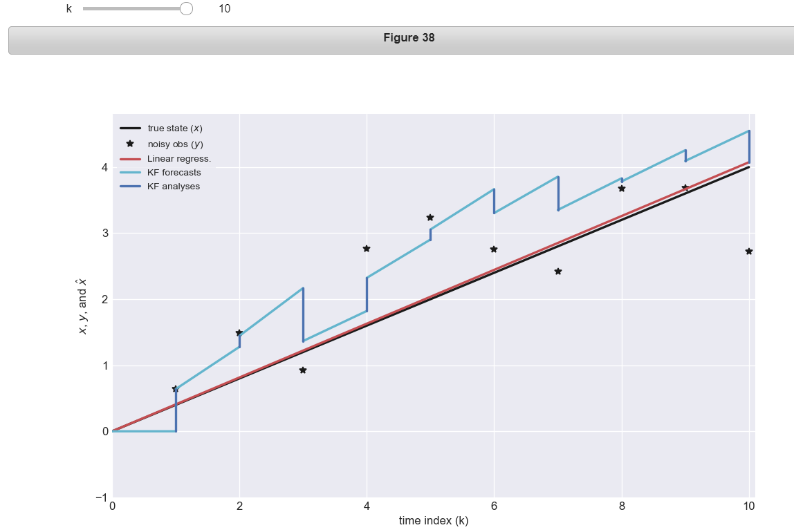
Visually: what is the relationship between the estimates provided by the KF and by linear regression?


T4 - Multivariate Kalman
prior(forcast):P(x),在预测步,求均值和方差

likelihood:P(y|x)
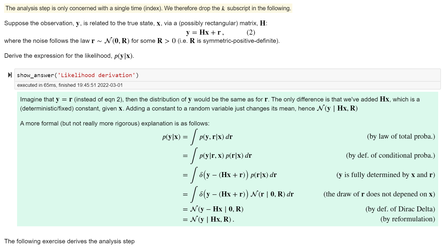
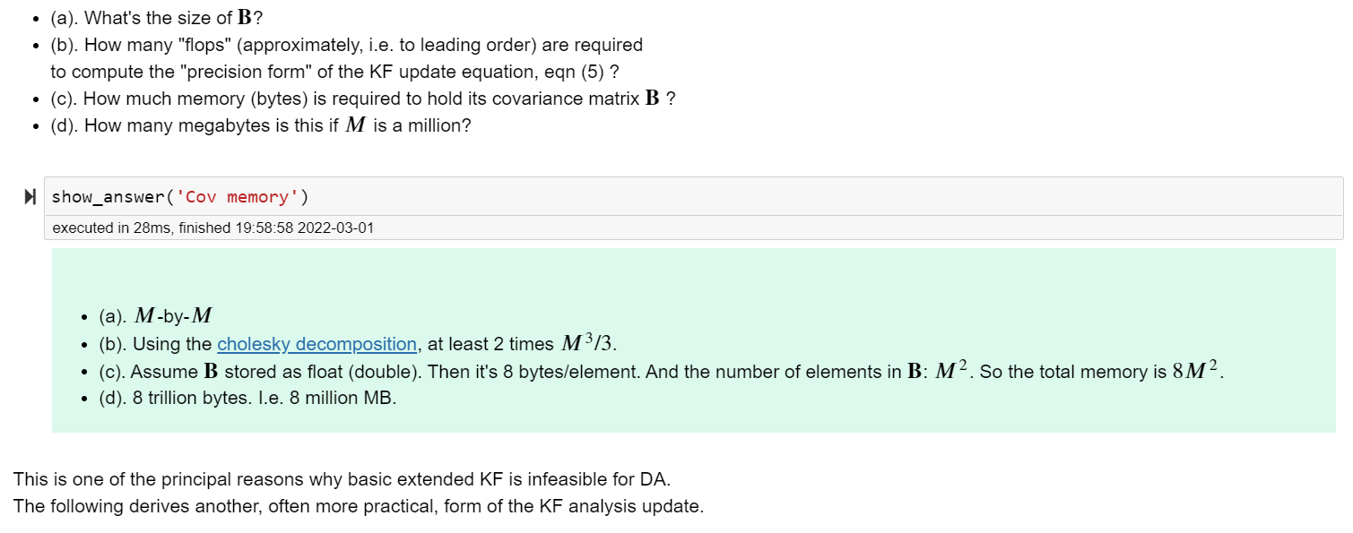
posterior(analysis):P(x|y),在分析步,The ‘precision’ form of the KF

↑ KF的precision形式

KF的precision形式的计算很昂贵
Sherman-Morrison-Woodbury lemma/identity

↑ SMW求逆公式

↑ SMW求逆公式对B,R,V,U的要求
SMW推论1

SMW推论2

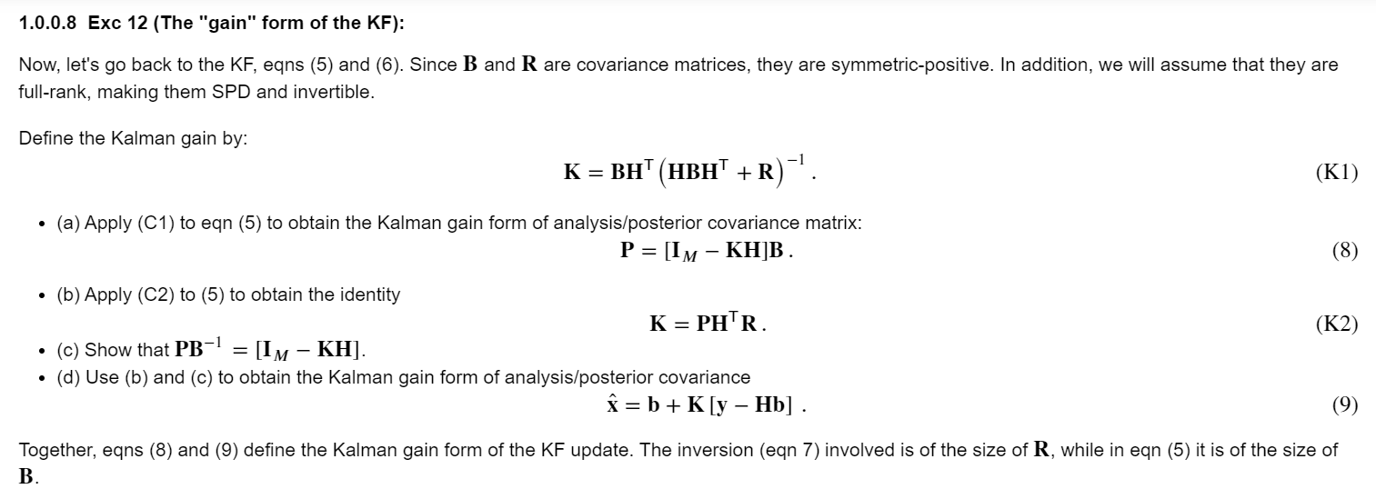
posterior(analysis):KF的gain形式
T5 - Time series analysis
The example model

Estimation by the Kalman filter (and smoother) with DAPPER
ValueError: path is on mount 'C:', start on mount 'D:'
在pycharm上运行~
AttributeError: 'NoneType' object has no attribute 'session'