07-阅读：DAPPER

No tag

数据同化

Publish Date: 2022-03-17

Update Date: 2024-07-29

Word Count: 8.5k

`<center>`参考资料：DAPPER `</center>`

必要信息

必要信息	文件位置
首次接触 DAPPER	`Liu-Jincan.github.io` 中的 `给定区域WW3试验（同化部分）`
添加到endnote文件夹	D盘 `数据同化`，检索，wjc老师
下载的DAPPER文件夹	D盘 `DAPPER-master` ，未保存到百度网盘
创建的DAPPER 博客	本博客

github官方仓库：https://github.com/nansencenter/DAPPER

Git托管（待）

SSSSSSSSSSSSSSSSSSSSSSSSSSSSSSSSSSSSSSSSSSSSSSSS

【README.md】

DAPPER is a set of templates for benchmarking the performance of data assimilation (DA) methods.

The tests provide experimental support and guidance for new developments in DA.

The typical set-up is a synthetic (twin) experiment, where you specify a dynamic model and an observational model, and use these to generate a synthetic truth (multivariate time series), and then estimate that truth given the models and noisy observations.

twin 实验

Getting started

Install, then read, run and try to understand examples/basic_{1,2,3}.py.

安装

Some of the examples can also be opened in Jupyter, and thereby run in the cloud (i.e. without installation, but requiring Google login): .

jupyter，colab

This screencast provides an introduction.

Youtube关于DAPPER的介绍视频

The documentation includes general guidelines and the API, but for any serious use you will want to read and adapt the code yourself.

DAPPER 文档/手册

If you use it in a publication, please cite, e.g., The experiments used (inspiration from) DAPPER [ref], version 1.2.1, where [ref] points to .

DAPPER 引用

Lastly, for an introduction to DA theory also using Python, see these tutorials.

一个关于DA理论的教程

Highlights

DAPPER enables the numerical investigation of DA methods through a variety of typical test cases and statistics. It

(a) reproduces numerical benchmarks results reported in the literature, and
(b) facilitates comparative studies,

thus promoting the (a) reliability and (b) relevance of the results. For example, this figure is generated by examples/basic_3.py and is a reproduction of figure 5.7 of these lecture notes.

In summary, it is well suited for teaching and fundamental DA research.

↑ DAPPER 适合教学和基础的DA研究

Also see its drawbacks.

↑ wjc老师上课讲的那本书~

DA methods

Method	Literature reproduced
EnKF `<sup>`1 `</sup>`	Sakov08, Hoteit15, Grudzien2020
EnKF-N	Bocquet12, Bocquet15
EnKS, EnRTS	Raanes2016
iEnKS / iEnKF / EnRML / ES-MDA `<sup>`2 `</sup>`	Sakov12, Bocquet12, Bocquet14
LETKF, local & serial EAKF	Bocquet11
Sqrt. model noise methods	Raanes2014
Particle filter (bootstrap)`<sup>`3 `</sup>`	Bocquet10
Optimal/implicit Particle filter `<sup>`3 `</sup>`	Bocquet10
NETF	Tödter15, Wiljes16
Rank histogram filter (RHF)	Anderson10
4D-Var
3D-Var
Extended KF
Optimal interpolation
Climatology
`<!-- markdownlint-restore -->`

1 : Stochastic, DEnKF (i.e. half-update), ETKF (i.e. sym. sqrt.).
Serial forms are also available.
Tuned with inflation and “random, orthogonal rotations”.

2 : Also supports the bundle version,
and “EnKF-N”-type inflation.

3 : Resampling: multinomial
(including systematic/universal and residual).
The particle filter is tuned with “effective-N monitoring”,
“regularization/jittering” strength, and more.

For a list of ready-made experiments with suitable,
tuned settings for a given method (e.g. the iEnKS), use:

grep -r "xp.*iEnKS" dapper/mods

Test cases (models)

Model	Lin	TLM**	PDE?	Phys.dim.	State len	Lyap≥0	Implementer
Id	Yes	Yes	No	N/A	*	0	Raanes
Linear Advect. (LA)	Yes	Yes	Yes	1d	1000 *	51	Evensen/Raanes
DoublePendulum	No	Yes	No	0d	4	2	Matplotlib/Raanes
Ikeda	No	Yes	No	0d	2	1	Raanes
LotkaVolterra	No	Yes	No	0d	5 *	1	Wikipedia/Raanes
Lorenz63	No	Yes	“Yes”	0d	3	2	Sakov
Lorenz84	No	Yes	No	0d	3	2	Raanes
Lorenz96	No	Yes	No	1d	40 *	13	Raanes
Lorenz96s	No	Yes	No	1d	10 *	4	Grudzien
LorenzUV	No	Yes	No	2x 1d	256 + 8 *	≈60	Raanes
LorenzIII	No	No	No	1d	960 *	≈164	Raanes
Vissio-Lucarini 20	No	Yes	No	1d	36 *	10	Yumeng
Kuramoto-Sivashinsky	No	Yes	Yes	1d	128 *	11	Kassam/Raanes
Quasi-Geost (QG)	No	No	Yes	2d	129²≈17k	≈140	Sakov

*: Flexible; set as necessary
**: Tangent Linear Model included?

The models are found as subdirectories within dapper/mods.

A model should be defined in a file named __init__.py,
and illustrated by a file named demo.py.

↑ 模型定义

Most other files within a model subdirectory
are usually named authorYEAR.py and define a HMM object,
which holds the settings of a specific twin experiment,

using that model,
as detailed in the corresponding author/year’s paper.
A list of these files can be obtained using

find dapper/mods -iname '[a-z]*[0-9]*.py'

Some files contain settings used by several papers.

Moreover, at the bottom of each such file should be (in comments)
a list of suitable, tuned settings for various DA methods,

↑ HMM 模型设置

along with their expected, average rmse.a score for that experiment.

↑ rmse.a 度量

As mentioned above, DAPPER reproduces literature results.
You will also find results that were not reproduced by DAPPER.

Installation

Works on Linux/Windows/Mac.

Prerequisite: Python>=3.7

If you’re an expert, setup a python environment however you like.

Otherwise: Install Anaconda, then open the Anaconda terminal and run the following commands:

conda create --yes --name dapper-env python=3.8
conda activate dapper-env
python --version

Ensure the printed version is 3.7 or more.

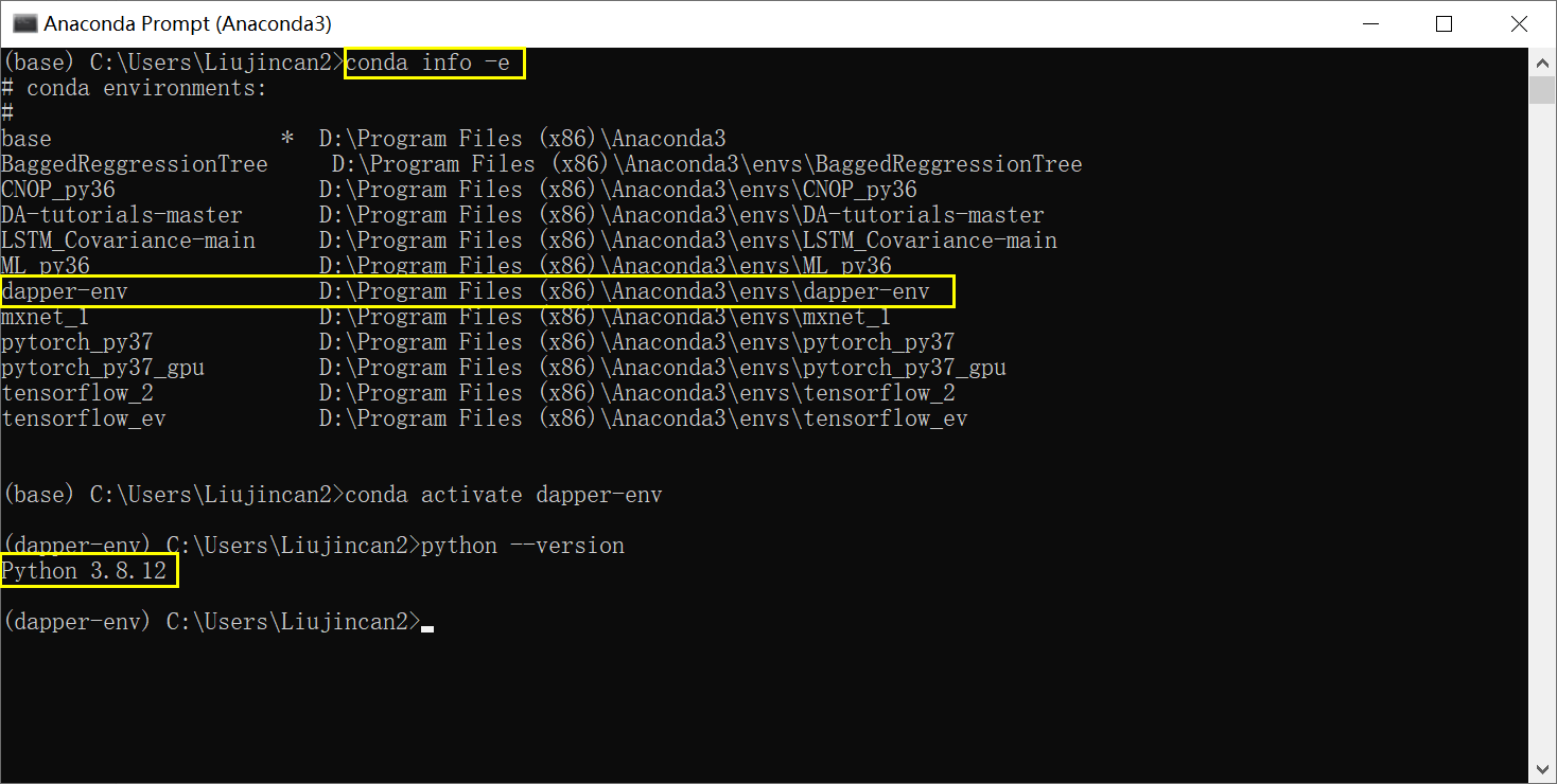
Keep using the same terminal for the commands below.

Install: for development（失败）

Install for development (recommended)

Do you want the DAPPER code available to play around with? Then

Download and unzip (or git clone) DAPPER.

链接：https://pan.baidu.com/s/1_W_6Ej4AP1fEVg6SEqXTXw
提取码：1234
–来自百度网盘超级会员V5的分享
Move the resulting folder wherever you like,
and cd into it (ensure you’re in the folder with a setup.py file).
pip install -e '.[dev]'
You can omit [dev] if you don’t need to do serious development.

下载总是出现错误~~

Install: as library（成功）

Install as library

Do you just want to run a script that requires DAPPER? Then

If the script comes with a requirements.txt file, then do
pip install -r path/to/requirements.txt.

setup.py的INSTALL_REQUIRES内容，作为requirements.txt的内容
If not, hopefully you know the version of DAPPER needed. Run
pip install dapper==1.0.0 to get version 1.2.3 (as an example).

Test the installation（成功）

You should now be able to do run your script with python path/to/script.py.
For example, if you are in the DAPPER dir,

python examples/basic_1.py

PS: If you closed the terminal (or shut down your computer), you’ll first need to run conda activate dapper-env

在pycharm中运行basic_1.py

Similar projects

DAPPER is aimed at research and teaching (see discussion up top). Example of limitations:

It is not suited for very big models (>60k unknowns).
Time-dependent error covariances and changes in lengths of state/obs (although the Dyn and Obs models may otherwise be time-dependent).
Non-uniform time sequences not fully supported.

The scope of DAPPER is restricted because

Moreover, even straying beyond basic configurability appears unrewarding when already building on a high-level language such as Python. Indeed, you may freely fork and modify the code of DAPPER, which should be seen as a set of templates, and not a framework.

↑ DAPPER 只是一个模板，不是框架

Also, DAPPER comes with no guarantees/support. Therefore, if you have an operational or real-world application, such as WRF, you should look into one of the alternatives, sorted by approximate project size.

↑ and ↓ 实际中的应用，WRF，替代？

Name	Developers	Purpose (approximately)
DART	NCAR	General
PDAF	AWI	General
JEDI	JCSDA (NOAA, NASA, ++)	General
OpenDA	TU Delft	General
EMPIRE	Reading (Met)	General
ERT	Statoil	History matching (Petroleum DA)
PIPT	CIPR	History matching (Petroleum DA)
MIKE	DHI	Oceanographic
OAK	Liège	Oceanographic
Siroco	OMP	Oceanographic
Verdandi	INRIA	Biophysical DA
PyOSSE	Edinburgh, Reading	Earth-observation DA

Below is a list of projects with a purpose more similar to DAPPER’s (research in DA, and not so much using DA):

↑ and ↓ 研究DA算法，却很少实际中用DA

Name	Developers	Notes
DAPPER	Raanes, Chen, Grudzien	Python
SANGOMA	Conglomerate*	Fortran, Matlab
hIPPYlib	Villa, Petra, Ghattas	Python, adjoint-based PDE methods
FilterPy	R. Labbe	Python. Engineering oriented.
DASoftware	Yue Li, Stanford	Matlab. Large inverse probs.
Pomp	U of Michigan	R
EnKF-Matlab	Sakov	Matlab
EnKF-C	Sakov	C. Light-weight, off-line DA
pyda	Hickman	Python
PyDA	Shady-Ahmed	Python
DasPy	Xujun Han	Python
DataAssim.jl	Alexander-Barth	Julia
DataAssimilationBenchmarks.jl	Grudzien	Julia, Python
Datum	Raanes	Matlab
IEnKS code	Bocquet	Python

The EnKF-Matlab and IEnKS codes have been inspirational in the development of DAPPER.

*: AWI/Liege/CNRS/NERSC/Reading/Delft

SSSSSSSSSSSSSSSSSSSSSSSSSSSSSSSSSSSSSSSSSSSSSSSS

【examples 文件夹】

README.md

Examples

Here are some example scripts using DAPPER. They all consist of one (or more) synthetic experiments.

Run them using python examples/the_script.py, or with the %run command inside ipython.

Some of the scripts have also been converted to Jupyter notebooks (.ipynb). You can try them out without installing anything by pressing this button (but note that some plotting features won’t work, and that it requires a Google login):

Description

basic_1.py: A single experiment, with Liveplotting.
basic_2.py: Comparison of several DA methods.
basic_3.py: Comparison of many DA methods and other experiment settings.
param_estim.py: Similar to basic_2, but with parameter estimation.
stoch_model1.py: A perfect-yet-random model, with various integration schemes.
stoch_models.py: As above, but studies the relationship between model uncertainty and numerical discretization error.

SSSSSSSSSSSSSSSSSSSSSSSSSSSSSSSSSSSSSSSSS

basic_1.py

run with python console

代码

# ## Illustrate usage of DAPPER to (interactively) run a synthetic ("twin") experiment.

# #### Imports
# <b>NB:</b> If you're on <mark><b>Gooble Colab</b></mark>,
# then replace `%matplotlib notebook` below by
# `!python -m pip install git+https://github.com/nansencenter/DAPPER.git` .
# Also note that liveplotting does not work on Colab.

导入包_nb_dpr_da_HMM=0
# %matplotlib notebook
from mpl_tools import is_notebook_or_qt as nb

import dapper as dpr
import dapper.da_methods as da

# #### Load experiment setup: the hidden Markov model (HMM)
from dapper.mods.Lorenz63.sakov2012 import HMM


生成随机数种子_seed=0
# #### Generate the same random numbers each time this script is run
seed = dpr.set_seed(3000)


生成实验的真实数据_xx和噪声_yy=0
# #### Simulate synthetic truth (xx) and noisy obs (yy)
HMM.tseq.T = 30  # shorten experiment
xx, yy = HMM.simulate()


生成实验的同化方法配置_xp=0
# #### Specify a DA method configuration ("xp" is short for "experiment")

# xp = da.OptInterp()
# xp = da.Var3D()
# xp = da.ExtKF(infl=90)
xp = da.EnKF('Sqrt', N=10, infl=1.02, rot=True)
xp = da.iEnKS('Sqrt', N=10, infl=1.02, rot=True)
# xp = da.PartFilt(N=100, reg=2.4, NER=0.3)



进行同化=0
# #### Assimilate yy, knowing the HMM; xx is used to assess the performance

#xp.assimilate(HMM, xx, yy, liveplots=not nb)
xp.assimilate(HMM, xx, yy, liveplots=False)


度量同化结果=0
# #### Average the time series of various statistics

xp.stats.average_in_time()

# #### Print some averages

print(xp.avrgs.tabulate(['rmse.a', 'rmv.a']))
print(xp.avrgs.tabulate(['err.rms.a', 'rmv.a']))
#print(xp.avrgs.tabulate(['err.m.a', 'rmv.a']))


再次显示=0
# #### Replay liveplotters
#xp.stats.replay()
#xp.stats.replay(
    # speed=.6
#)

# #### Further diagnostic plots

if nb:
    import dapper.tools.viz as viz
    viz.plot_rank_histogram(xp.stats)
    viz.plot_err_components(xp.stats)
    viz.plot_hovmoller(xx)

# #### Explore objects

if nb:
    print(xp)

if nb:
    print(HMM)

if nb:
    # print(xp.stats) # quite long printout
    print(xp.avrgs)



QT_为什么再次显示的图形不如直接生成的图形光滑=0
# #### Excercise: Why are the replay plots not as smooth as the liveplot?
# *Hint*: provide the keyword `store_u=True` to `assimilate()` to avoid this.




QT_为什么再次显示的图形仅包含蓝线=0
# #### Excercise: Why does the replay only contain the blue lines?





EX_尝试另一个DA方法_iEnKS_liveplots设置=0
# #### Excercise: Try out each of the above DA methods (currently commented out).
# Next, remove the call to `replay`, and set `liveplots=False` above.
# Now, use the iterative EnKS (`iEnKS`), and try to find a parameter combination
# for it so that you achieve a lower `rmse.a` than with the `PartFilt`.
#


QT_如何调参=0
# *Hint*: In general, there is no free lunch. Similarly, not all methods work
# for all problems;
#
# additionally, methods often have parameters that require
# tuning. Luckily, in DAPPER, you should be able to find suitably tuned
# configuration settings for various DA methods *in the files that define the
# HMM*.
#
# If you do not find a suggested configuration for a given method, you
# will have to tune it yourself.
#
# The example script `basic_2` shows how DAPPER
# facilitates the tuning process, and `basic_3` takes this further.


EX_尝试不同的模型HMM=0
# #### Excercise: Run an experiment for each of these models
# - LotkaVolterra
# - Lorenz96
# - LA
# - QG



EX_尝试不同的度量方法=0
# #### Excercise: Printing other diagnostics.
# - Create a new code cell, and copy-paste the above `print(...tabulate)`
#   command into it. Then, replace `rmse` by `err.rms`. This should yield
#   the same printout, as is merely an abbreviation of the latter.
#
# - Next, figure out how to print the time average *forecast (i.e. prior)* error
#   (and `rmv`) instead. Explain (in broad terms) why the values are larger than
#   for the *analysis* values.
#
# - Finally, instead of the `rms` spatial/field averages,
#   print the regular mean (`.m`) averages. Explain why `err.m` is nearly zero,
#   in contrast to `err.rms`.

QT：EX_尝试不同的度量方法

不理解部分：Next, figure out how to print the time average forecast (i.e. prior) error (and rmv) instead. Explain (in broad terms) why the values are larger than for the analysis values.

知道了：同化后，添加了观测信息，肯定误差变小了呀~~

SSSSSSSSSSSSSSSSSSSSSSSSSSSSSSSS

basic_lorenz63_detail.py （为了更好地理解，自己做的一个函数）

basic_2.py

# ## Illustrate usage of DAPPER to benchmark multiple DA methods.

# #### Imports
# <b>NB:</b> If you're on <mark><b>Gooble Colab</b></mark>,
# then replace `%matplotlib notebook` below by
# `!python -m pip install git+https://github.com/nansencenter/DAPPER.git` .
# Also note that liveplotting does not work on Colab.


导入包_dpr_da=0
# %matplotlib notebook
import dapper as dpr
import dapper.da_methods as da

导入动力模型lorenz63_HMM=0
# #### DA method configurations
# hidden Markov model (HMM)
from dapper.mods.Lorenz63.sakov2012 import HMM  # Expected rmse.a:


手册_xpList=0  #https://nansencenter.github.io/DAPPER/dapper/xp_launch.html#dapper.xp_launch.xpList
xps = dpr.xpList()

手册_baseline同化方法=0
xps += da.Climatology()                                      # 7.6
xps += da.OptInterp()                                        # 1.25
xps += da.Persistence()                                      # 10.7
xps += da.PreProg(lambda k, xx, yy: xx[k])                   # 0
xps += da.Var3D(xB=0.1)                                      # 1.03

手册_extended同化方法=0
xps += da.ExtKF(infl=90)                                     # 0.87

手册_ensemble同化方法=0
xps += da.EnKF('Sqrt'   , N=3   , infl=1.30)                 # 0.82
xps += da.EnKF('Sqrt'   , N=10  , infl=1.02, rot=True)       # 0.63
xps += da.EnKF('PertObs', N=500 , infl=0.95, rot=False)      # 0.56
xps += da.EnKF_N(         N=10             , rot=True)       # 0.54

手册_variational同化方法=0
xps += da.iEnKS('Sqrt'  , N=10  , infl=1.02, rot=True)       # 0.31

手册_particleFilter同化方法=0
xps += da.PartFilt(       N=100 , reg=2.4  , NER=0.3)        # 0.38
xps += da.PartFilt(       N=800 , reg=0.9  , NER=0.2)        # 0.28
# xps += da.PartFilt(       N=4000, reg=0.7  , NER=0.05)       # 0.27
# xps += da.PFxN(xN=1000,   N=30  , Qs=2     , NER=0.2)        # 0.56


EX_导入动力模型lorenz96_HMM=0
# #### With Lorenz-96 instead

# +
# from dapper.mods.Lorenz96.sakov2008 import HMM   # Expected rmse.a:
# xps = dpr.xpList()
# xps += da.Climatology()                                     # 3.6
# xps += da.OptInterp()                                       # 0.95
# xps += da.Var3D(xB=0.02)                                    # 0.41
# xps += da.ExtKF(infl=6)                                     # 0.24
# xps += da.EnKF('PertObs', N=40, infl=1.06)                  # 0.22
# xps += da.EnKF('Sqrt'   , N=28, infl=1.02, rot=True)        # 0.18
# # More sophisticated:
# xps += da.EnKF_N(         N=24, rot=True)                   # 0.21
# xps += da.EnKF_N(         N=24, rot=True, xN=2)             # 0.18
# xps += da.iEnKS('Sqrt'  , N=40, infl=1.01, rot=True)        # 0.17
# # With localisation:
# xps += da.LETKF(          N=7 , infl=1.04, rot=True, loc_rad=4)  # 0.22
# xps += da.SL_EAKF(        N=7 , infl=1.07, rot=True, loc_rad=6)  # 0.23
# -

EX_导入其它动力模型_HMM=0
# #### Other models (suitable xp's listed in HMM files):

# +
# from dapper.mods.LA           .evensen2009 import HMM
# from dapper.mods.KS           .bocquet2019 import HMM
# from dapper.mods.LotkaVolterra.settings101 import HMM
# -

xps_launch操作=0
# #### Launch

# Write some more non-arg parameters to the `xps`. In this case we set the seed,
# so that repeat experiments produce exactly the same result.
for xp in xps:
    xp.seed = 3000

# Adjust experiment duration
HMM.tseq.T = 50

# Run/assimilate (for each `xp` in `xps`)
save_as = xps.launch(HMM, liveplots=False)

# #### Print results
print(xps.tabulate_avrgs())

basic_3a.py

SSSSSSSSSSSSSSSSSSSSSSSSSSSSSSSSSSSSSSSSSSSSSSSS

【dapper 文件夹：对应的是手册】

手册网站：https://nansencenter.github.io/DAPPER/dapper/index.html#gsc.tab=0

Usage

See README/Getting-started

Then, adapt one of the example scripts to your needs. Make sure you have a working adaptation examples/basic_1.py before adapting basic_2 and basic_3.

↑ go-to~

Since the generality of DAPPER is limited it is quite likely you will also need to make changes to the DAPPER code itself.

If, in particular, you wish to illustrate and run benchmarks with your own model or method, then

If it is a complex one, you may be better off using DAPPER merely as inspiration (but you can still cite it) rather than trying to squeeze everything into its templates.

↑ DAPPER的局限性
If it is relatively simple, however, you may well want to use DAPPER. In that case, read this:
- dapper.mods
- dapper.da_methods
↑ DAPPER的两个核心模块：mods，da_methods

Developer guide

Features

The main features are listed in README/highlights. Additionally, there is:

Parallelisation:
- (Independent) experiments can run in parallel; see examples/basic_3.py
- Forecast parallelisation is possible since the (user-implemented) model has access to the full ensemble; see example in dapper.mods.QG.
- Analysis parallelisation over local domains; see example in LETKF
Classes that simplify treating:
- Experiment administration and launch via xpList and data processing and presentation via xpSpace.
- Time sequences use via Chronology and Ticker.
- Random variables via RV: Gaussian, Student-t, Laplace, Uniform, …, as well as support for custom sampling functions.
- Covariance matrices via CovMat: provides input flexibility/overloading, lazy eval that facilitates the use of non-diagonal covariance matrices (whether sparse or full).
Diagnostics and statistics with
- Confidence interval on times series (e.g. rmse) averages with
  - automatic correction for autocorrelation
  - significant digits printing
- Automatic averaging of several types for sub-domains (e.g. “ocean”, “land”, etc.)

↑ DAPPER的特点

API reference

The rendered docstrings can be browsed through the following links, which are also available in the left sidebar.

"""Data Assimilation with Python: a Package for Experimental Research

.. include:: ./README.md
"""

__version__ = "1.3.0"

# A parsimonious list of imports used in the examples
from .dpr_config import rc
from .tools.datafiles import find_latest_run, load_xps
from .tools.rounding import round2sigfig
from .tools.seeding import set_seed
from .xp_launch import combinator, seed_and_simulate, xpList
from .xp_process import xpSpace


# Exclude "demo.py" files from documentation.
# NB: pdoc complains/warns that it cannot find these files,
# but it still works fine. https://github.com/pdoc3/pdoc/issues/206
def _find_demos(as_path=False):
    """Discover all model demo.py scripts."""
    lst = []
    for d in (rc.dirs.dapper/"mods").iterdir():
        x = d/"demo.py"
        if x.is_file():
            x = x.relative_to(rc.dirs.DAPPER)
            if not as_path:
                x = str(x.with_suffix("")).replace("/", ".")
            lst.append(x)
    return lst


__pdoc__ = {k: False for k in _find_demos()}

↑ 参考的API，能够全面了解dapper，实现对dapper的应用

SSSSSSSSSSSSSSSSSSSSSSSSSSSSSSSSSSSSSSSSSSSSSSSS

dapper.da_methods

Contains the data assimilation methods included with DAPPER …

See the README section on DA Methods for an overview of the methods included with DAPPER.

Defining your own method

Follow the example of one of the methods within one of the sub-directories/packages. The simplest example is perhaps EnKF.

General advice for programming/debugging scientific experiments

Start with something simple. This helps make sure the basics of the experiment are reasonable. For example, start with
- a pre-existing example,
- something you are able to reproduce,
- a small/simple model.
  - Set the observation error to be small.
  - Observe everything.
  - Don’t include model error and/or noise to begin with.
Additionally, test a simple/baseline method to begin with. When including an ensemble method, start with using a large ensemble, and introduce localisation later.
Take incremental steps towards your ultimate experiment setup. Validate each incremental setup with prints/plots. If results change, make sure you understand why.
Use short experiment duration. You probably don’t need statistical significance while debugging.

SSSSSSSSSSSSSSSSSSSSSSSSSSSSSSSSSSSSSSSSSSSSSSSS

dapper.da_methods.baseline

Unsophisticated” but robust (widely applicable) DA methods …

Many are based on raanes2016thesis.

Raanes, Patrick N 2016 Improvements to ensemble methods for data assimilation in the geosciences (PhD thesis). University of Oxford.

"""Unsophisticated" but robust (widely applicable) DA methods.

Many are based on `bib.raanes2016thesis`.
"""
from typing import Callable, Optional

import numpy as np

import dapper.tools.series as series
from dapper.stats import center
from dapper.tools.linalg import mrdiv
from dapper.tools.matrices import CovMat
from dapper.tools.progressbar import progbar

from . import da_method


@da_method()
class Climatology:
    """A baseline/reference method.

    Note that the "climatology" is computed from truth, which might be
    (unfairly) advantageous if the simulation is too short (vs mixing time).
    """

    def assimilate(self, HMM, xx, yy):
        muC = np.mean(xx, 0)
        AC  = xx - muC
        PC  = CovMat(AC, 'A')

        self.stats.assess(0, mu=muC, Cov=PC)
        self.stats.trHK[:] = 0

        for k, ko, _, _ in progbar(HMM.tseq.ticker):
            fau = 'u' if ko is None else 'fau'
            self.stats.assess(k, ko, fau, mu=muC, Cov=PC)


@da_method()
class OptInterp:
    """Optimal Interpolation -- a baseline/reference method.

    Uses the Kalman filter equations,
    but with a prior from the Climatology.
    """

    def assimilate(self, HMM, xx, yy):
        Id = np.eye(HMM.Nx)

        # Compute "climatological" Kalman gain
        muC = np.mean(xx, 0)
        AC  = xx - muC
        PC  = (AC.T @ AC) / (xx.shape[0] - 1)

        # Setup scalar "time-series" covariance dynamics.
        # ONLY USED FOR DIAGNOSTICS, not to affect the Kalman gain.
        L  = series.estimate_corr_length(AC.ravel(order='F'))
        SM = fit_sigmoid(1/2, L, 0)

        # Init
        mu = muC
        self.stats.assess(0, mu=mu, Cov=PC)

        for k, ko, t, dt in progbar(HMM.tseq.ticker):
            # Forecast
            mu = HMM.Dyn(mu, t-dt, dt)
            if ko is not None:
                self.stats.assess(k, ko, 'f', mu=muC, Cov=PC)

                # Analysis
                H  = HMM.Obs.linear(muC, t)
                KG  = mrdiv(PC@H.T, H@PC@H.T + HMM.Obs.noise.C.full)
                mu = muC + KG@(yy[ko] - HMM.Obs(muC, t))

                P  = (Id - KG@H) @ PC
                SM = fit_sigmoid(P.trace()/PC.trace(), L, k)

            self.stats.assess(k, ko, mu=mu, Cov=2*PC*SM(k))


@da_method()
class Var3D:
    """3D-Var -- a baseline/reference method.

    This implementation is not "Var"-ish: there is no *iterative* optimzt.
    Instead, it does the full analysis update in one step: the Kalman filter,
    with the background covariance being user specified, through B and xB.
    """

    B: Optional[np.ndarray] = None
    xB: float               = 1.0

    def assimilate(self, HMM, xx, yy):
        Id = np.eye(HMM.Nx)
        if isinstance(self.B, np.ndarray):
            # compare ndarray 1st to avoid == error for ndarray
            B = self.B.astype(float)
        elif self.B in (None, 'clim'):
            # Use climatological cov, estimated from truth
            B = np.cov(xx.T)
        elif self.B == 'eye':
            B = Id
        else:
            raise ValueError("Bad input B.")
        B *= self.xB

        # ONLY USED FOR DIAGNOSTICS, not to change the Kalman gain.
        CC = 2*np.cov(xx.T)
        L  = series.estimate_corr_length(center(xx)[0].ravel(order='F'))
        P  = HMM.X0.C.full
        SM = fit_sigmoid(P.trace()/CC.trace(), L, 0)

        # Init
        mu = HMM.X0.mu
        self.stats.assess(0, mu=mu, Cov=P)

        for k, ko, t, dt in progbar(HMM.tseq.ticker):
            # Forecast
            mu = HMM.Dyn(mu, t-dt, dt)
            P  = CC*SM(k)

            if ko is not None:
                self.stats.assess(k, ko, 'f', mu=mu, Cov=P)

                # Analysis
                H  = HMM.Obs.linear(mu, t)
                KG = mrdiv(B@H.T, H@B@H.T + HMM.Obs.noise.C.full)
                mu = mu + KG@(yy[ko] - HMM.Obs(mu, t))

                # Re-calibrate fit_sigmoid with new W0 = Pa/B
                P = (Id - KG@H) @ B
                SM = fit_sigmoid(P.trace()/CC.trace(), L, k)

            self.stats.assess(k, ko, mu=mu, Cov=P)


def fit_sigmoid(Sb, L, kb):
    """Return a sigmoid [function S(k)] for approximating error dynamics.

    We use the logistic function for the sigmoid; it's the solution of the
    "population growth" ODE: dS/dt = a*S*(1-S/S(∞)).
    NB: It might be better to use the "error growth ODE" of Lorenz/Dalcher/Kalnay,
    but this has a significantly more complicated closed-form solution,
    and reduces to the above ODE when there's no model error (ODE source term).

    The "normalized" sigmoid, S1, is symmetric around 0, and S1(-∞)=0 and S1(∞)=1.

    The sigmoid S(k) = S1(a*(k-kb) + b) is fitted (see docs/snippets/sigmoid.jpg) with

    - a corresponding to a given corr. length L.
    - b to match values of S(kb) and Sb
    """

    def sigmoid(k): return 1/(1+np.exp(-k))  # normalized sigmoid
    def inv_sig(s): return np.log(s/(1-s))  # its inverse

    a = 1/L
    b = inv_sig(Sb)

    def S(k):
        return sigmoid(b + a*(k-kb))

    return S


@da_method()
class Persistence:
    """Sets estimate to the **true state** at the previous time index.

    The analysis (.a) stat uses the previous obs. time.
    The forecast and universal (.f and .u) stats use previous integration time index.
    """

    def assimilate(self, HMM, xx, yy):
        prev = xx[0]
        self.stats.assess(0, mu=prev)
        for k, ko, _t, _dt in progbar(HMM.tseq.ticker):
            self.stats.assess(k, ko, 'fu', mu=xx[k-1])
            if ko is not None:
                self.stats.assess(k, ko, 'a', mu=prev)
                prev = xx[k]


@da_method()
class PreProg:
    """Simply look-up the estimates in user-specified function (`schedule`).

    For example, with `schedule` given by `lambda k, xx, yy: xx[k]`
    the error (err.rms, err.ma, ...) should be 0.
    """

    schedule: Callable
    tag: str = None

    def assimilate(self, HMM, xx, yy):
        self.stats.assess(0, mu=self.schedule(0, xx, yy))
        for k, ko, _t, _dt in progbar(HMM.tseq.ticker):
            self.stats.assess(k, ko, 'fu', mu=self.schedule(k, xx, yy))
            if ko is not None:
                self.stats.assess(k, ko, 'a', mu=self.schedule(k, xx, yy))

函数：fit_sigmoid

Return a sigmoid [function S(k)] for approximating error dynamics.

Climatology

A baseline/reference method.

Note that the “climatology” is computed from truth, which might be (unfairly) advantageous if the simulation is too short (vs mixing time).

QT: climatology???

OptInterp

Optimal Interpolation – a baseline/reference method.

Uses the Kalman filter equations, but with a prior from the Climatology.

Var3D

3D-Var – a baseline/reference method.

This implementation is not “Var”-ish: there is no iterative optimzt. Instead, it does the full analysis update in one step: the Kalman filter, with the background covariance being user specified, through B and xB.

Persistence

Sets estimate to the true state at the previous time index.

The analysis (.a) stat uses the previous obs. time. The forecast and universal (.f and .u) stats use previous integration time index.

PreProg

Simply look-up the estimates in user-specified function (schedule).

For example, with schedule given by lambda k, xx, yy: xx[k] the error (err.rms, err.ma, …) should be 0.

SSSSSSSSSSSSSSSSSSSSSSSSSSSSSSSSSSSSSSSSSSSSSSSS

dapper.da_methods.ensemble

The EnKF and other ensemble-based methods.

EnKF

The ensemble Kalman filter.

Refs: evensen2009ensemble.

Evensen, G 2009 The ensemble Kalman filter for combined state and parameter estimation. Control Systems, IEEE, 29(3): 83–104.

EnKS

The ensemble Kalman smoother.

Refs: evensen2009ensemble

同EnKF

The only difference to the EnKF is the management of the lag and the reshapings.

EnRTS

EnRTS (Rauch-Tung-Striebel) smoother.

Refs: raanes2016thesis

Raanes, Patrick N 2016 Improvements to ensemble methods for data assimilation in the geosciences (PhD thesis). University of Oxford.

SL_EAKF

Serial, covariance-localized EAKF.

Refs: karspeck2007experimental.

Karspeck, A R and Anderson, J L 2007 Experimental implementation of an ensemble adjustment filter for an intermediate ENSO model. Journal of Climate, 20(18): 4638–4658.

In contrast with LETKF, this iterates over the observations rather than over the state (batches).

Used without localization, this should be equivalent (full ensemble equality) to the EnKF with upd_a='Serial'.

LETKF

Same as EnKF (Sqrt), but with localization.

Refs: hunt2007efficient.

Hunt, B R, Kostelich, E J, and Szunyogh, I 2007 Efficient data assimilation for spatiotemporal chaos: A local ensemble transform Kalman filter. Physica D: Nonlinear Phenomena, 230(1): 112–126.

NB: Multiproc. yields slow-down for dapper.mods.Lorenz96, even with batch_size=(1,). But for dapper.mods.QG (batch_size=(2,2) or less) it is quicker.

NB: If len(ii) is small, analysis may be slowed-down with ‘-N’ infl.

EnKF_N

This implementation is pedagogical, prioritizing the “dual” form. In consequence, the efficiency of the “primal” form suffers a bit. The primal form is included for completeness and to demonstrate equivalence. In iEnKS, however, the primal form is preferred because it already does optimization for w (as treatment for nonlinear models).

SSSSSSSSSSSSSSSSSSSSSSSSSSSSSSSSSSSSSSSSSSSSSSSS

dapper.da_methods.extended

The extended KF (EKF) and the (Rauch-Tung-Striebel) smoother.

ExtKF

The extended Kalman filter.

If everything is linear-Gaussian, this provides the exact solution to the Bayesian filtering equations.

ExtRTS

The extended Rauch-Tung-Striebel (or “two-pass”) smoother.

SSSSSSSSSSSSSSSSSSSSSSSSSSSSSSSSSSSSSSSSSSSSSSSS

dapper.da_methods.other

More experimental or esoteric DA methods.

RHF

Rank histogram filter.

Refs: anderson2010non.

Quick & dirty implementation without attention to (de)tails.

LNETF

The Nonlinear-Ensemble-Transform-Filter (localized).

Refs: wiljes2016second, todter2015second.

It is (supposedly) a deterministic upgrade of the NLEAF of lei2011moment.

SSSSSSSSSSSSSSSSSSSSSSSSSSSSSSSSSSSSSSSSSSSSSSSS

dapper.da_methods.particle

Weight- & resampling-based DA methods.

PartFilt

Particle filter ≡ Sequential importance (re)sampling SIS (SIR).

Refs: wikle2007bayesian, van2009particle, chen2003bayesian

This is the bootstrap version: the proposal density is just

OptPF

‘Optimal proposal’ particle filter, also known as ‘Implicit particle filter’.

Ref: bocquet2010beyond.

Note: Regularization (Qs) is here added BEFORE Bayes’ rule.

If Qs==0: OptPF should be equal to the bootstrap filter PartFilt.

PFa

PF with weight adjustment withOUT compensating for the bias it introduces.

‘alpha’ sets wroot before resampling such that N_effective becomes >alpha*N.

Using alpha≈NER usually works well.

Explanation: Recall that the bootstrap particle filter has “no” bias, but significant variance (which is reflected in the weights). The EnKF is quite the opposite. Similarly, by adjusting the weights we play on the bias-variance spectrum.

NB: This does not mean that we make a PF-EnKF hybrid – we’re only playing on the weights.

Hybridization with xN did not show much promise.

PFxN_EnKF

Particle filter with EnKF-based proposal, q.

Also employs xN duplication, as in PFxN.

Recall that the proposals: Opt.: q_n(x) = c_n·N(x|x_n,Q )·N(y|Hx,R) (1) EnKF: q_n(x) = c_n·N(x|x_n,bar{B})·N(y|Hx,R) (2) with c_n = p(y|x^{k-1}_n) being the composite proposal-analysis weight, and with Q possibly from regularization (rather than actual model noise).

Here, we will use the posterior mean of (2) and cov of (1). Or maybe we should use x_a^n distributed according to a sqrt update?

PFxN

Particle filter with buckshot duplication during analysis.

Idea: sample xN duplicates from each of the N kernels. Let resampling reduce it to N.

Additional idea: employ w-adjustment to obtain N unique particles, without jittering.

SSSSSSSSSSSSSSSSSSSSSSSSSSSSSSSSSSSSSSSSSSSSSSSS

dapper.da_methods.variational

Variational DA methods (iEnKS, 4D-Var, etc).

iEnKS

Iterative EnKS.

Special cases: EnRML, ES-MDA, iEnKF, EnKF raanes2019revising.

As in bocquet2014iterative, optimization uses Gauss-Newton. See bocquet2012combining for Levenberg-Marquardt. If MDA=True, then there’s not really any optimization, but rather Gaussian annealing.

Var4D

4D-Var.

Cycling scheme is same as in iEnKS (i.e. the shift is always 1*ko).

This implementation does NOT do gradient decent (nor quasi-Newton) in an inner loop, with simplified models. Instead, each (outer) iteration is computed non-iteratively as a Gauss-Newton step. Thus, since the full (approximate) Hessian is formed, there is no benefit to the adjoint trick (back-propagation). => This implementation is not suited for big systems.

Incremental formulation is used, so the formulae look like the ones in iEnKS.

SSSSSSSSSSSSSSSSSSSSSSSSSSSSSSSSSSSSSSSSSSSSSSSS

dapper.da_config

Load default and user configurations into the rc dict …

The rc dict can be updated (after startup) as any normal dict. See the source for the default configuration.

crtl+/，pycharm，批量注释

修改了data的路径

"""Load default and user configurations into the `rc` dict.

The `rc` dict can be updated (after startup) as any normal dict. See the
[source](https://github.com/nansencenter/DAPPER/blob/master/dapper/dpr_config.yaml)
for the default configuration.
"""

import os
from pathlib import Path

import matplotlib as mpl
import yaml
from mpl_tools import is_using_interactive_backend
from struct_tools import DotDict


##################################
# Load configurations
##################################
dapper_dir = Path(__file__).absolute().parent
#dapper_dir = Path('__file__').absolute().parent
rc = DotDict()
rc.loaded_from = []
for d in [dapper_dir, "~", "~/.config", "."]:
    d = Path(d).expanduser().absolute()
    for prefix in [".", ""]:
        f = d / (prefix+"dpr_config.yaml")
        if f.is_file():
            dct = yaml.load(open(f), Loader=yaml.SafeLoader)
            rc.loaded_from.append(str(f))
            if dct:
                if d == dapper_dir:
                    rc.update(dct)
                else:
                    for k in dct:
                        if k in rc:
                            rc[k] = dct[k]
                        else:
                            print(f"Warning: invalid key '{k}' in '{f}'")


##################################
设置路径=0
# Setup dir paths
##################################
rc.dirs = DotDict()
rc.dirs.dapper = dapper_dir
rc.dirs.DAPPER = rc.dirs.dapper.parent
# Data path
# x = rc.pop("data_root")
# if x.lower() in ["$cwd", "$pwd"]:
#     x = Path.cwd()
# elif x.lower() == "$dapper":
#     x = rc.dirs.DAPPER
# else:
#     x = Path(x)

x = rc.dirs.DAPPER
rc.dirs.data = x / "dpr_data"
rc.dirs.samples = rc.dirs.data / "samples"

# Expanduser, create dir
for d in rc.dirs:
    rc.dirs[d] = rc.dirs[d].expanduser()
    os.makedirs(rc.dirs[d], exist_ok=True)


##################################
# Disable rc.liveplotting in case of non-interactive backends
##################################
# Otherwise, warnings are thrown on every occurence of plt.pause
# (though not plot_pause), and (who knows) maybe errors too.
# Also, the assimilation slows down, even though nothing is shown.
LP = rc.liveplotting
if LP and not is_using_interactive_backend():
    # Note: plot_pause could maybe be adapted to also work for
    # "inline" backend (which is not striclty interactive), but I think
    # this would be buggy, and is incompatible with a "stop" button.
    print("\nWarning: You have not disableed interactive/live plotting",
          "in your dpr_config.yaml,",
          "but this is not supported by the current matplotlib backend:",
          f"{mpl.get_backend()}. To enable it, try using another backend.\n")
    LP = False
rc.liveplotting = LP

SSSSSSSSSSSSSSSSSSSSSSSSSSSSSSSSSSSSSSSSSSSSSSSS

dapper.mods

Models included with DAPPER …

请参阅关于测试用例(模型)的README部分，以获得DAPPER中包含的模型的概述。

这些模型都很简单;这有助于提高实验结果的可靠性、可重复性和可归因性。

定义自己的模型

以“dapper/mods”文件夹中的一个模型为例。本质上，你只需要定义一个“HiddenMarkovModel”的所有属性。为了确保这是有效的，我们建议以下结构:

创建一个目录:my_model
创建一个文件:my_model/__init__.py，在其中定义模型的核心工作。
- 通常，这在 step(x, t, dt)函数中结束，它定义了从一个时间t到另一个时间t + dt的状态x的动态模型/系统映射。他的模型“operator”必须支持2d阵列(即集成)和1d阵列(单实现)输入，并返回与输入相同维数的输出。See:
  - dapper.mods.Lorenz63: use of ens_compatible.
  - dapper.mods.Lorenz96: use of relatively clever slice notation.
  - dapper.mods.LorenzUV:use of cleverer slice notation: … (ellipsis). Consider pre-defining the slices like so:
```
iiX = (..., slice(None, Nx))
iiP = (..., slice(Nx, None))
```
    to abbreviate the indexing elsewhere.
  - dapper.mods.QG: use of parallelized for loop (map).
  ↑ 感觉好难呀
- 可选：定义一个建议/示例初始状态x0。这有助于说明不同合成实验的初始条件，因为随机变量以x0为中心。将系统大小指定为len(x0)也是一种方便的方法。在许多实验中，x0的具体值并不重要，因为大多数系统是混乱的，并且统计的平均值只计算time> BurnIn > 0，如果实验足够长，它将不依赖于x0。尽管如此，在吸引器或盆地上预先定义一个点通常是很方便的，或至少确保“物理”，以便更快地旋转(老化)。
- 可选：定义一个被调用的数字 Tplot，该数字定义诊断的实时绘图使用的（滑动）时间窗口。
- 可选：要使用（扩展）卡尔曼滤波器或 4D-Var，您需要定义模型线性化，通常称为 dstep_dx. 注意：这里只需要支持一维输入（单实现）
大多数模型是使用基于程序和函数的样式定义的。但是，dapper.mods.LorenzUV并 dapper.mods.QG使用 OOP。当要研究不同的控制变量设置时，这更加灵活和稳健，并且更适合。

在参数估计问题中，参数被视为“前向模型”的输入变量。这不一定需要 OOP。见 examples/param_estim.py。
制作文件：my_model/demo.py直观地展示模型的模拟，并验证它是否正常工作。

首先，测试模型是否适用于 1 个实现，然后运行多个（同时）。此外，在使用更有效/更冒险的时间步之前，从一个小的积分时间步开始。请注意，同化的时间步长可能需要更短，因为它可能会导致不稳定。
理想情况下，两者 my_model/__init__.py都不 my_model/demo.py 依赖于 DAPPER dapper.mods之外的组件。
创建一个文件:my_model/my_settings_1.py，它定义了(或“配置”，因为通常很少进行实际编程)一个完整的隐马尔可夫模型，用于合成实验(也称为“孪生实验”或OSSE)。关于这需要什么，请参阅HiddenMarkovModel 每个现有的模型都有几个文献中模型设置的例子。看，例如，dapper.mods.Lorenz63.sakov2012。

这些配置并不一定具有很高的编程标准，因为它们可能是为了复制某些实验而在短时间内匆忙创建的，并不是为了重用。

然而，有时它们会被另一个配置脚本重用，从而导致一个主要的陷阱:对导入的HMM(或模型的模块本身)所做的更改也会影响原始对象(因为它们是可变的，因此会被引用)。这通常不是问题，因为很少会导入两个或更多单独的配置。然而，测试套件导入了所有的配置，这些配置可能会无意间交互。为了避免这种情况，您应该在对HMM进行任何更改之前使用HMM的复制方法。

一旦你做了一些实验,你认为值得注意的你应该添加一个评论中“建议设置/调优”部分的底部my_model / my_settings_1.py清单的一些相关DA方法配置测试,随着RMSE(或其他数据),你获得了这些方法。在DAPPER中已经有很多例子，用于与文献交叉引用，以验证DAPPER的工作方式(以及出版物的可复制性)。

HiddenMarkovModel(HMM)

隐马尔可夫模型(HMM)的容器。

这应该包含运行合成DA实验所需的细节，也被称为“孪生实验”，或**OSSE(观察系统模拟实验)**。然后可以通过运行HiddenMarkovModel.simulate()来获得合成的事实和观测结果。

更多细节请参见示例中的脚本。

Dyn 算子

Obs 算子

Operator

Container for the dynamical and the observational maps.

SSSSSSSSSSSSSSSSSSSSSSSSSSSSSSSSSSSSSSSSSSSSSSSS

dapper.stats

Statistics for the assessment of DA methods …

SSSSSSSSSSSSSSSSSSSSSSSSSSSSSSSSSSSSSSSSSSSSSSSS

dapper.tools

If the only tool you have is a hammer, it’s hard to eat spaghetti.

rounding

round2sigfig函数

Round to significant figures.

datafiles

create_run_dir函数

Validate save_as and create dir rc.dirs.data / save_as and sub-dirs.

The data gets saved here unless save_as is False/None.

Note: multiprocessing (locally or in the cloud) requires saving/loading data.

from dapper.dpr_config import rc

seeding

set_seed函数

本质上是rnd.seed(sd)，但也返回sd。

rnd.seed()的缺点是它产生的RandomState不能用简单的seed表示(映射的seed - >状态是非满射的)。相反，当sd在[None， “clock”]， set_seed()从时间(微秒)生成一个种子，然后可以返回。

如果sd==False:什么都不做。

**为什么种子管理?**它使随机实验的重现性成为可能。此外，在比较实验中，对每一种方法使用相同的种子可以产生一种“方差减少”的形式，例如。CRN,参考维基百科。这种CRN技巧通常有助于加速比较，但不应在出版物中使用，出版物应该简单地使用聚合统计。

**为什么我们使用全局生成器?**因为这是我们习惯的。我们并不担心线程安全。

**为什么DAPPER中的许多地方使用sd=3000 ?**因为我喜欢这个数字。例如:“André 3000”，“我爱你3000”。

SSSSSSSSSSSSSSSSSSSSSSSSSSSSSSSSSSSSSSSSSSSSSSSS

dapper.xp_launch

Tools (notably xpList) for setup and running of experiments (known as xps) …

See create_run_dir() for documentation save_as.

combinator函数

通过组合param_dict中的值列表来大量创建xp。

返回一个函数(for_params)，该函数为给定的da_method()创建所有可能的参数组合(从参数值列表中)。这比依赖于xpList的unique要高效得多。参数

在给定的DA方法的参数中找不到的会被for_params忽略。
指定为关键字for_params的值，防止使用param_dict中相应的值列表(如果有)

Beware! If, eg., infl or rot are in param_dict, aimed at the EnKF, but you forget that they are also attributes some method where you don’t actually want to use them (eg. SVGDF), then you’ll create many more than you intend.

run_experiment函数

Used by xpList.launch() to run each single (DA) experiment (“xp”).

This involves steps similar to examples/basic_1.py, i.e.:

setup : Initialize experiment.
xp.assimilate : run DA, pass on exception if fail_gently
xp.stats.average_in_time : result averaging
xp.avrgs.tabulate : result printing
dill.dump : result storage

参数：

setup

这个函数必须接受两个参数:HMM和xp，并返回DA方法要使用的HMM(通常与输入HMM相同，但可以修改)，以及(通常是合成的)真值和obs时间序列。

这让你能够在批量启动的实验中定制单个实验的几乎任何方面(即不仅仅是DA的参数)。方法)。通常你会抓取一个或多个参数值存储在xp(参阅da_method())，并对它们进行操作，通常是通过将它们分配给一些影响实验的对象。因此，通过为每个这样的参数值生成一个新的xp，您可以调查结果对该参数的影响/敏感性。例子包括:
- 设置种子。查看默认设置，即seed_and_simulation()，了解如何或应该如何完成。
- 设置HMM的某些方面，比如观测噪声，或者观测间隔。这可以通过以下方法实现:
```
def setup(hmm, xp):
    hmm.Obs.noise = GaussRV(M=hmm.Nx, C=xp.obs_noise)
    hmm.tseq.dkObs = xp.time_between_obs
    import dapper as dpr
    return dpr.seed_and_simulate(hmm, xp)
```
  这个过程可能涉及更多的步骤,例如从一个数据文件加载一个完整的协方差矩阵,作为obs_noise指定的参数,分配到c之前还要注意,import语句并不是必需的(假设衣冠楚楚的已经进口的外范围,通常是主要的脚本),除非在远程服务器上运行实验。
  
  有时，您想要设置的参数不能作为HMM的常规属性之一访问。例如，洛伦兹-96模型中的力。在这种情况下，你可以将这些行添加到setup函数中:
```
import dapper.mods.Lorenz96 as core
core.Force = xp.the_force_parameter
```
  但是，如果您的模型是一个OOP实例，那么导入方法将不起作用，因为它将为您提供原始的模型实例，而setup()将处理它的一个副本。相反，您可以在setup()中重新初始化整个模型，并覆盖HMM.Dyn。然而，在启动实验之前，将实例分配给一些自定义属性可能会更容易一些，例如HMM.Dyn.object = the_model_instance，这使您能够在setup()中设置HMM.Dyn.object的参数。请注意，这种方法不适用于模块(例如，结合上面的例子，HMM.Dyn.object = core)，因为模块是不可序列化的。
- 使用完全不同的HMM来生成truth/obs (xx/yy)，而不是DA将使用的HMM。或者从文件中加载truth/obs时间序列。在这两种情况下，您可能还必须在返回xx和yy之前对它们进行一些裁剪或切片。

dapper.tools.datafiles.create_run_dir

seed_and_simulate

Default experiment setup (sets seed and simulates truth and obs).

Used by xpList.launch() via run_experiment().

HMM.simulate?

SSSSSSSSSSSSSSSSSSSSSSSSSSSSSSSSSSSSSSSSSSSSSSSS

dapper.xp_process

Tools (notably xpSpace) for processing and presenting experiment data.

Jincan

https://Liu-Jincan.github.io/2022/03/17/yan-jiu-sheng-justtry-function/endnote-shu-ju-tong-hua/08-code-dapper/

All articles in this blog are used except for special statements CC BY 4.0 reprint policy. If reproduced, please indicate source Jincan !

No tag

研一下-云计算合稿

2022-03-21 研究生JustTry

研一下-海表面风和海浪多源数据融合实况

2022-03-05 研究生JustTry

07-阅读：DAPPER

<center>参考资料：DAPPER </center>

必要信息

Git托管（待）

【README.md】

Getting started

Highlights

DA methods

Test cases (models)

Installation

Prerequisite: Python>=3.7

Install: for development（失败）

Install: as library（成功）

Test the installation（成功）

Similar projects

【examples 文件夹】

README.md

basic_1.py

QT：EX_尝试不同的度量方法

basic_lorenz63_detail.py （为了更好地理解，自己做的一个函数）

basic_2.py

basic_3a.py

【dapper 文件夹：对应的是手册】

Usage

Developer guide

Features

API reference

dapper.da_methods

Defining your own method

General advice for programming/debugging scientific experiments

dapper.da_methods.baseline

QT: climatology???

dapper.da_methods.ensemble

dapper.da_methods.extended

dapper.da_methods.other

dapper.da_methods.particle

dapper.da_methods.variational

dapper.da_config

dapper.mods

定义自己的模型

HiddenMarkovModel(HMM)

Dyn 算子

Obs 算子

dapper.stats

dapper.tools

rounding

datafiles

create_run_dir函数

seeding

dapper.xp_launch

run_experiment函数

dapper.xp_process

Thanks for your reward

`<center>`参考资料：DAPPER `</center>`